Penumbra is a fully private proof-of-stake network and decentralized exchange for the Cosmos ecosystem.
Penumbra integrates privacy with proof-of-stake through a novel private delegation mechanism that provides staking derivatives, tax-efficient staking, and on-chain governance with private voting. Penumbra connects to the Cosmos ecosystem via IBC, acting as an ecosystem-wide shielded pool and allowing private transactions in any IBC-compatible asset. Users can also swap these assets using ZSwap, a private decentralized exchange supporting sealed-bid batch auctions and Uniswap-v3-style concentrated liquidity. Sealed-bid batch auctions prevent frontrunning, provide better execution, and reveal only the net flow across a pair of assets in each block, and liquidity positions are created anonymously, allowing traders to approximate their desired trading function without revealing their individual beliefs about prices.
This website renders the work-in-progress protocol specification for Penumbra.
Press s or use the magnifying glass icon for full-text search.
If you’re interested in technical discussion about the project, why not
- join the discord,
- check out the repo and issue tracker,
- view the roadmap goals,
- or follow the project on Twitter for updates.
Private Transactions
Penumbra records all value in a single multi-asset shielded pool based on the Zcash Sapling design, but allows private transactions in any kind of IBC asset. Inbound IBC transfers shield value as it moves into the zone, while outbound IBC transfers unshield value.
Unlike Zcash, Penumbra has no notion of transparent transactions or a
transparent value pool; instead, inbound IBC transfers are analogous to t2z
Zcash transactions, outbound IBC transfers are analogous to z2t Zcash
transactions, and the entire Cosmos ecosystem functions analogously to
Zcash’s transparent pool.
Unlike the Cosmos Hub or many other chains built on the Cosmos SDK, Penumbra has no notion of accounts. Only validators have any kind of long-term identity, and this identity is only used (in the context of transactions) for spending the validator’s commission.
Private Staking
In a proof-of-stake system like the Cosmos Hub, stakeholders delegate staking tokens by bonding them to validators. Validators participate in Tendermint consensus with voting power determined by their delegation size, and delegators receive staking rewards in exchange for taking on the risk of being penalized for validator misbehavior (slashing).
Integrating privacy and proof of stake poses significant challenges. If delegations are public, holders of the staking token must choose between privacy on the one hand and staking rewards and participation in consensus on the other hand. Because the majority of the stake will be bonded to validators, privacy becomes an uncommon, opt-in case. But if delegations are private, issuing staking rewards becomes very difficult, because the chain no longer knows the amount and duration of each address’ delegations.
Penumbra sidesteps this problem using a new mechanism that eliminates staking rewards entirely, treating unbonded and bonded stake as separate assets, with an epoch-varying exchange rate that prices in what would be a staking reward in other systems. This mechanism ensures that all delegations to a particular validator are fungible, and can be represented by a single delegation token representing a share of that validator’s delegation pool, in effect a first-class staking derivative. Although delegation fungibility is key to enabling privacy, as a side effect, delegators do not realize any income while their stake is bonded, only a capital gain (or loss) on unbonding.
The total amount of stake bonded to each validator is part of the public chain state and determines consensus weight, but the delegation tokens themselves are each just another token to be recorded in a multi-asset shielded pool. This provides accountability for validators and privacy and flexibility for delegators, who can trade and transact with their delegation tokens just like they can with any other token.
It also provides an alternate perspective on the debate between fixed-supply and inflation-based rewards. Choosing the unbonded token as the numéraire, delegators are rewarded by inflation for taking on the risk of validator misbehavior, and the token supply grows over time. Choosing (a basket of) delegation tokens as the numéraire, non-delegators are punished by depreciation for not taking on any risk of misbehavior, and the token supply is fixed.
Private Governance
Like the Cosmos Hub, Penumbra supports on-chain governance with delegated voting. Unlike the Cosmos Hub, Penumbra’s governance mechanism supports secret ballots. Penumbra users can anonymously propose votes by escrowing a deposit of bonded stake. Stakeholders vote by proving ownership of their bonded stake prior to the beginning of the voting period and encrypting their votes to a threshold key controlled by the validator set. Validators sum encrypted votes and decrypt only the per-epoch totals.
Private DEX
Penumbra provides private batch swaps using ZSwap. ZSwap allows users to privately swap between any pair of assets. Individual swaps publicly burn their input notes and privately mint their output notes. All swaps in each block are executed in a single batch. Users can also provide liquidity by anonymously creating concentrated liquidity positions. These positions reveal the amount of liquidity and the bounds in which it is concentrated, but are not otherwise linked to any identity, so that (with some care) users can privately approximate arbitrary trading functions without revealing their specific views about prices.
Concepts and Mechanisms
This section provides an overview of the concepts involved in Penumbra’s mechanism design.
Validators
Validators in Penumbra undergo various transitions depending on chain activity.
                                 ┌────────────────────────────────────────────────────────────────────────────┐
                                 │                                                                            │
                                 │            ┌ ─ ─ ─ ─ ─ ─ ─ ─ ─ ─                                           │
                                 │              Genesis Validator  │                                          │
                                 │            │                             ┏━━━━━━━━━━━━━━━━━━━━━━━┓         │
                                 │             ─ ─ ─ ─ ─ ─ ─ ─ ─ ─ ┘        ┃      Tombstoned       ┃         │
                                 │                       │          ┌──────▶┃     (Misbehavior)     ┃         │
                                 │                       │          │       ┗━━━━━━━━━━━━━━━━━━━━━━━┛         │
                                 │                       │          │                                         │
┌ ─ ─ ─ ─ ─ ─ ─ ─ ─ ─            │                       ▼          │                                         ▼
      Validator      │      ┏━━━━━━━━━┓              ╔══════╗       │                                   ┏━━━━━━━━━━━┓
│     Definition     ──────▶┃Inactive ┃─────────────▶║Active║───────┼────────────────────────────────┬─▶┃ Disabled  ┃
   (in transaction)  │      ┗━━━━━━━━━┛              ╚══════╝       │                                │  ┗━━━━━━━━━━━┛
└ ─ ─ ─ ─ ─ ─ ─ ─ ─ ─            ▲                                  │       ┏━━━━━━━━━━━━━━━━━━━━━┓  │        │
                                 │                                  └──────▶┃ Jailed (Inactivity) ┃──┘        │
                                 │                                          ┗━━━━━━━━━━━━━━━━━━━━━┛           │
                                 │                                                     │                      │
                                 └─────────────────────────────────────────────────────┴──────────────────────┘
Single lines represent unbonded stake, and double lines represent bonded stake.
Validators become known to the chain either at genesis, or by means of a transaction with a ValidatorDefinition action in them. Validators transition through five states:
- Inactive: a validator whose delegation pool is too small to participate in consensus set
- Active: a validator whose delegation pool is large enough to participate in consensus and must meet uptime requirements
- Jailed: a validator that has been slashed and removed from consensus for downtime, that may return later
- Tombstoned: a validator that has been permanently slashed and removed from consensus for byzantine misbehavior and may not return
- Disabled: a validator that has been manually disabled by the operator, that may return to
Inactivelater
Validators specified in the genesis config begin in the active state, with whatever stake was allocated to their delegation pool at genesis. Otherwise, new validators begin in the inactive state, with no stake in their delegation pool. At this point, the validator is known to the chain, and stake can be contributed to its delegation pool. Stake contributed to an inactive validator’s delegation pool does not earn rewards (the validator’s rates are held constant), but it is also not bonded, so undelegations are effective immediately, with no unbonding period and no output quarantine.
The chain chooses a validator limit N as a consensus parameter. When a validator’s delegation pool (a) has a nonzero balance and (b) its (voting-power-adjusted) size is in the top N validators, it moves into the active state during the next epoch transition. Active validators participate in consensus, and are communicated to Tendermint. Stake contributed to an active validator’s delegation pool earns rewards (the validator’s rates are updated at each epoch to track the rewards accruing to the pool). That stake is bonded, so undelegations have an unbonding period and an output quarantine. An active validator can exit the consensus set in four ways.
First, the validator could be jailed and slashed for inactivity. This can happen in any block, triggering an unscheduled epoch transition. Jailed validators are immediately removed from the consensus set. The validator’s rates are updated to price in the slashing penalty, and are then held constant. Validators jailed for inactivity are not permanently prohibited from participation in consensus, and their operators can re-activate them by re-uploading the validator definition. Stake cannot be delegated to a slashed validator. Stake already contributed to a slashed validator’s delegation pool will enter an unbonding period to hold the validator accountable for any byzantine behavior during the unbonding period. Re-delegations may occur after the validator enters the “Inactive” state.
Second, the validator could be tombstoned and slashed for byzantine misbehavior. This can happen in any block, triggering an unscheduled epoch transition. Tombstoned validators are immediately removed from the consensus set. Any pending undelegations from a slashed validator are cancelled: the quarantined output notes are deleted, and the quarantined nullifiers are removed from the nullifier set. The validator’s rates are updated to price in the slashing penalty, and are then held constant. Tombstoned validators are permanently prohibited from participation in consensus (though their operators can create new identity keys, if they’d like to). Stake cannot be delegated to a tombstoned validator. Stake already contributed to a tombstoned validator’s delegation pool is not bonded (the validator has already been slashed and tombstoned), so undelegations are effective immediately, with no unbonding period and no quarantine.
Third, the validator could be manually disabled by the operator. The validator is then in the disabled state. It does not participate in consensus, and the stake in its delegation pool does not earn rewards (the validator’s rates are held constant). The stake in its delegation pool will enter an unbonding period at the time the validator becomes disabled. The only valid state a disabled validator may enter into is “inactive”, if the operator re-activates it by updating the validator definition.
Fourth, the validator could be displaced from the validator set by another validator with more stake in its delegation pool. The validator is then in the inactive state. It does not participate in consensus, and the stake in its delegation pool does not earn rewards (the validator’s rates are held constant). The stake in its delegation pool will enter an unbonding period at the time the validator becomes inactive. Inactive validators have three possible state transitions:
- they can become active again, if new delegations boost its weight back into the top N;
- they can be tombstoned, if evidence of misbehavior arises during the unbonding period;
- they can be disabled, if the operator chooses.
If (2) occurs, the same state transitions as in regular tombstoning occur: all pending undelegations are cancelled, etc. If (3) occurs, the unbonding period continues and the validator enters the disabled state. If (1) occurs, the validator stops unbonding, and all delegations become bonded again.
Batching Flows
Penumbra’s ledger records value as it moves between different economic roles – for instance, movement between unbonded stake and delegation tokens, movement between different assets as they are traded, etc. This creates a tension between the need to reveal the total amount of value in each role as part of the public chain state, and the desire to shield value amounts in individual transactions.
To address this tension, Penumbra provides a mechanism to aggregate value flows across a batch of transactions, revealing only the total amount and not the value contributed by each individual transaction. This mechanism is built using an integer-valued homomorphic encryption scheme that supports threshold decryption, so that the network’s validators can jointly control a decryption key.
Transactions that contribute value to a batch contain an encryption of the amount. To flush the batch, the validators sum the ciphertexts from all relevant transactions to compute an encryption of the batch total, then jointly decrypt it and commit it to the chain.
This mechanism doesn’t require any coordination between the users whose transactions are batched, but it does require that the validators create and publish a threshold decryption key. To allow batching across block boundaries, Penumbra organizes blocks into epochs, and applies changes to the validator set only at epoch boundaries. Decryption keys live for the duration of the epoch, allowing value flows to be batched over any time interval from 1 block up to the length of an epoch. We propose epoch boundaries on the order of 1-3 days.
At the beginning of each epoch, the validator set performs distributed key generation to produce a decryption key jointly controlled by the validators (on an approximately stake-weighted basis) and includes the encryption key in the first block of the epoch.
Because this key is only available after the first block of each epoch, some transactions cannot occur in the first block itself. Assuming a block interval similar to the Cosmos Hub, this implies an ~8-second processing delay once per day, a reasonable tradeoff against the complexity of phased setup procedures.
Addresses and Keys
Value transferred on Penumbra is sent to shielded payment addresses; these addresses are derived from spending keys through a sequence of intermediate keys that represent different levels of attenuated capability:
flowchart BT
    subgraph Address
    end;
    subgraph DTK[Detection Key]
    end;
    subgraph IVK[Incoming Viewing Key]
    end;
    subgraph OVK[Outgoing Viewing Key]
    end;
    subgraph FVK[Full Viewing Key]
    end;
    subgraph SK[Spending Key]
    end;
    subgraph SeedPhrase[Seed Phrase]
    end;

    index(address index);
    div{ };

    SeedPhrase --> SK;
    SK --> FVK;
    FVK --> OVK;
    FVK --> IVK;

    index --> div;
    IVK ----> div;
    div --> Address & DTK;
    DTK --> Address;
From bottom to top:
- the seed phrase is the root key material. Multiple wallets - each with separate spend authority - can be derived from this root seed phrase.
- the spending key is the capability representing spending authority for a given wallet;
- the full viewing key represents the capability to view all transactions related to the wallet;
- the outgoing viewing key represents the capability to view only outgoing transactions, and is used to recover information about previously sent transactions;
- the incoming viewing key represents the capability to view only incoming transactions, and is used to scan the block chain for incoming transactions.
Penumbra allows the same account to present multiple, publicly unlinkable addresses, keyed by an 16-byte address index. Each choice of address index gives a distinct shielded payment address. Because these addresses share a common incoming viewing key, the cost of scanning the blockchain does not increase with the number of addresses in use.
Finally, Penumbra also allows outsourcing probabilistic transaction detection to third parties using fuzzy message detection. Each address has a detection key; a third party can use this key to detect transactions that might be relevant to that key. Like a Bloom filter, this detection has false positives but no false negatives, so detection will find all relevant transactions, as well as some amount of unrelated cover traffic. Unlike incoming viewing keys, detection keys are not shared between diversified addresses, allowing fine-grained control of delegation.
This diagram shows only the user-visible parts of the key hierarchy. Internally, each of these keys has different components, described in detail in the Addresses and Keys chapter.
Privacy Implications
Users should be aware that giving out multiple detection keys to a detection entity can carry a subset of the privacy implications, described in Addresses and Detection Keys.
Assets and Amounts
Penumbra’s shielded pool can record arbitrary assets. To be precise, we define:
- an amount to be an untyped quantity of some asset;
- an asset type to be an ADR001-style denomination trace uniquely identifying a cross-chain asset and its provenance, such as:
denom(native chain A asset)transfer/channelToA/denom(chain B representation of chain A asset)transfer/channelToB/transfer/channelToA/denom(chain C representation of chain B representation of chain A asset)
- an asset ID to be a fixed-size hash of an asset type;
- a value to be a typed quantity, i.e., an amount and an asset id.
Penumbra deviates slightly from ADR001 in the definition of the asset ID. While ADR001 defines the IBC asset ID as the SHA-256 hash of the denomination trace, Penumbra hashes to a field element, so that asset IDs can be more easily used inside of a zk-SNARK circuit.
Notes, Nullifiers, and Trees
Transparent blockchains operate as follows: all participants maintain a copy of the (consensus-determined) application state. Transactions modify the application state directly, and participants check that the state changes are allowed by the application rules before coming to consensus on them.
On a shielded blockchain like Penumbra, however, the state is fragmented across all users of the application, as each user has a view only of their “local” portion of the application state recording their funds. Transactions update a user’s state fragments privately, and use a zero-knowledge proof to prove to all other participants that the update was allowed by the application rules.
Penumbra’s transaction model is derived from the Zcash shielded transaction design, with modifications to support multiple asset types, and several extensions to support additional functionality. The Zcash model is in turn derived from Bitcoin’s unspent transaction output (UTXO) model, in which value is recorded in transaction outputs that record the conditions under which they can be spent.
In Penumbra, value is recorded in notes, which function similarly to UTXOs. Each note specifies (either directly or indirectly) a type of value, an amount of value of that type, a spending key that authorizes spending the note’s value, and a unique nullifier derived from the note’s contents.
However, unlike UTXOs, notes are not recorded as part of the public chain state. Instead, the chain contains a state commitment tree, an incremental Merkle tree containing (public) commitments to (private) notes. Creating a note involves creating a new note commitment, and proving that it commits to a valid note. Spending a note involves proving that the spent note was previously included in the state commitment tree, using the spending key to demonstrate spend authorization, and revealing the nullifier, which prevents the same note from being spent twice. Nullifiers that correspond to each spent note are tracked in the nullifier set, which is recorded as part of the public chain state.
Transactions
Transactions describe an atomic collection of changes to the ledger state. Each transaction consists of a sequence of descriptions for various actions1. Each description adds or subtracts (typed) value from the transaction’s value balance, which must net to zero.
Penumbra adapts Sapling’s Spend, which spends a note and adds to the transaction’s value balance, and Output, which creates a new note and subtracts from the transaction’s value balance. Penumbra also adds many new descriptions to support additional functionality:
Transfers
-
Spend descriptions spend an existing note, adding its value to the transaction’s value balance;
-
Output descriptions create a new note, subtracting its value from the transaction’s value balance;
-
Transfer descriptions transfer value out of Penumbra by IBC, consuming value from the transaction’s value balance, and producing an ICS20
FungibleTokenPacketDatafor the counterparty chain;
Staking
-
Delegate descriptions deposit unbonded stake into a validator’s delegation pool, consuming unbonded stake from the transaction’s value balance and producing new notes recording delegation tokens representing the appropriate share of the validator’s delegation pool;
-
Undelegate descriptions withdraw from a validator’s delegation pool, consuming delegation tokens from the transaction’s value balance and producing new notes recording the appropriate amount of unbonded stake;
Governance
-
CreateProposal descriptions are used to propose measures for on-chain governance and supply a deposit, consuming bonded stake from the transaction’s value balance and producing a new note that holds the deposit in escrow;
-
WithdrawProposal descriptions redeem an escrowed proposal deposit, returning it to the transaction’s value balance and immediately withdrawing the proposal.
-
Vote descriptions perform private voting for on-chain governance and declare a vote. This description leaves the value balance unchanged.
Trading
-
Swap descriptions perform the first phase of a swap, consuming tokens of one type from a transaction’s value balance, burning them, and producing a swap commitment for use in the second stage;
-
SwapClaim descriptions perform the second phase of a swap, allowing a user who burned tokens of one type to mint tokens of the other type at the chain-specified clearing price, and adding the new tokens to a transaction’s value balance;
Market-making
-
OpenPosition descriptions open concentrated liquidity positions, consuming value of the traded types from the transaction’s value balance and adding the specified position to the AMM state;
-
ClosePosition descriptions close concentrated liquidity positions, removing the specified position to the AMM state and adding the value of the position, plus any accumulated fees or liquidity rewards, to the transaction’s value balance.
Each transaction also contains a fee specification, which is always transparently encoded. The value balance of all of a transactions actions, together with the fees, must net to zero.
Note that like Zcash Orchard, we use the term “action” to refer to one of a number of possible state updates; unlike Orchard, we do not attempt to conceal which types of state updates are performed, so our Action is an enum.
Governance
Penumbra supports on-chain governance with delegated voting. Validators’ votes are public and act as default votes for their entire delegation pool, while delegators’ votes are private, and override the default vote provided by their validator.
Votes are similar to Cosmos Hub: Yes, No, and Abstain have the same meanings.
However, Penumbra does not have NoWithVeto; instead, a sufficiently high threshold
of “no” votes (determined by a chain parameter) will slash a proposal, which causes
its deposit to be burned. This functions as a spam deterrent.
Proposals
Penumbra users can propose votes by escrowing a minimum amount of PEN. They
do this by creating a transaction with a ProposalSubmit description, which
consumes some amount of PEN from the transaction’s balance, and creates a
proposal_N_voting NFT, which can be redeemed for the proposal deposit in the case
that the voting concludes without slashing the proposal (both failed and passed
proposals can reclaim their deposit).
Proposals can either be normal or emergency proposals. In either case, the voting period begins immediately, in the next block after the proposal has been committed to the chain. Normal proposals have a fixed-length voting period, while emergency proposals are accepted as soon as a 1/3 majority of the stake is reached.
Because validators provide default votes for their delegation pool, an emergency proposal can in principle be accepted immediately, without any input from delegators. This allows time-critical resolution of emergencies (e.g., deploying an 0day hotfix); a 1/3 + 1 plurality of the stake required is already sufficient to halt the chain.
Proposals can also be withdrawn by their proposer prior to the end of the voting
period. This is done by creating a transaction with a ProposalWithdraw
description, and allows the community to iterate on proposals as the (social)
governance process occurs. For instance, a chain upgrade proposal can be
withdrawn and re-proposed with a different source hash if a bug is discovered
while upgrade voting is underway. Withdrawn proposals cannot be accepted, even
if the vote would have passed, but they can be slashed.1
Voting
Stakeholder votes are of the form , representing the weights for yes, no, and abstain, respectively. Most stakeholders would presumably set all but one weight to . Stakeholders vote by proving ownership of some amount of bonded stake (their voting power) prior to the beginning of the voting period.
To do this, they create a transaction with a Vote description. This
description identifies the validator and the proposal, proves spend
authority over a note recording dPEN(v), and reveals the note’s nullifier.
Finally, it proves vote consistency , produces a new
note with dPEN(v), and includes , an encryption
of the vote weights to the validators’ decryption key.
The proof statements in a Vote description establishing spend authority over
the note are almost identical to those in a Spend description. However, there
are two key differences. First, rather than checking the note’s
nullifier against the global nullifier set and marking it as spent, the
nullifier is checked against a snapshot of the nullifier set at the time that
voting began (establishing that it was unspent then), as well as against a
per-proposal nullifier set (establishing that it has not already been used for
voting). In other words, instead of marking that the note has been spent in
general, we only mark it as having been spent in the context of voting on a
specific proposal. Second, the ZK proof additionally proves that the note was
created before the proposal started, and the stateful checks ensure that it was not
spent after the proposal started.
This change allows multiple proposals to be voted on concurrently, at the cost
of linkability. While the same note can be used to vote on multiple proposals,
those votes, as well as the subsequent spend of the note, will have the same
nullifier and thus be linkable to each other. However, the Vote descriptions
are shielded, so an observer only learns that two opaque votes were related to
each other.
We suggest that wallets roll over the note the first time it is used for voting
by creating a transaction with Vote, Spend, and Output descriptions. This
mitigates linkability between Vote and Spend descriptions, and means that
votes on any proposals created after the first vote are unlinkable from prior
votes.
Counting Votes
At the end of each epoch, validators collect the encrypted votes from each delegation pool, aggregate the encrypted votes into encrypted tallies and decrypt the tallies. These intermediate tallies are revealed, because it is not possible to batch value flows over time intervals longer than one epoch. In practice, this provides a similar dynamic as existing (transparent) on-chain governance schemes, where tallies are public while voting is ongoing.
At the end of the voting period, the per-epoch tallies are summed. For each validator , the votes for each option are summed to determine the portion of the delegation pool that voted; the validator’s vote acts as the default vote for the rest of the delegation pool. Finally, these per-validator subtotals are multiplied by the voting power adjustment function to obtain the final vote totals.
If the vote was not slashed, the proposal_N_voting NFT created during proposal
submission can be redeemed for the original proposal deposit (if not slashed)
and a commemorative proposal_N_passed, proposal_N_failed, or proposal_N_slashed
NFT.
If withdrawing a proposal halted on-chain voting immediately, the escrow mechanism would not be effective at deterring spam, since the proposer could yank their proposal at the last minute prior to losing their deposit. However, at the UX level, withdrawn proposals can be presented as though voting were closed, since validators’ default votes are probably sufficient for spam deterrence.
Primitives
Penumbra uses the following cryptographic primitives, described in the following sections:
-
The Proof System section describes the choice of proving curve (BLS12-377) and proof system (Groth16, and potentially PLONK in the future);
-
The
decaf377section describesdecaf377, a parameterization of the Decaf construction defined over the BLS12-377 scalar field, providing a prime-order group that can be used inside or outside of a circuit; -
The Poseidon for BLS12-377 section describes parameter selection for an instantiation of Poseidon, a SNARK-friendly sponge construction, over the BLS12-377 scalar field;
-
The Fuzzy Message Detection section describes a construction that allows users to outsource a probabilistic detection capability, allowing a third party to scan and filter the chain on their behalf, without revealing precisely which transactions are theirs.
-
The Homomorphic Threshold Decryption section describes the construction used to batch flows of value across transactions.
-
The Randomizable Signatures section describes
decaf377-rdsa, a variant of the Zcash RedDSA construction instantiated overdecaf377, used for binding and spend authorization signatures. -
The Key Agreement section describes
decaf377-ka, an instantiation of Diffie-Hellman key agreement overdecaf377.
Proving Considerations
Penumbra needs SNARK proofs. Because the choice of proving system and proving curve can’t really be cleanly separated from the rest of the system choices (e.g., the native field of the proving system informs what embedded curve is available, and how circuit programming is done), large parts of the rest of the system design block on making a choice of proving system.
Goals
-
Near-term implementation availability. We’d like to ship a useful product first, and iterate and expand it later.
-
High performance for fixed functionality. Penumbra intends to support fixed functionality initially; programmability is a good future goal but isn’t a near-term objective. The fixed functionality should have as high performance as possible.
-
Longer-term flexibility. The choice should ideally not preclude many future choices for later functionality. More precisely, it should not impose high switching costs on future choices.
-
Recursion capability. Penumbra doesn’t currently make use of recursion, but there are a lot of interesting applications it could be used for.
Setup ceremonies are beneficial to avoid for operational reasons, but not for security reasons. A decentralized setup procedure is sufficient for security.
Options
Proof systems:
- Groth16:
- Pros: high performance, very small proofs, mature system
- Cons: requires a setup for each proof statement
- PLONK:
- Pros: universal setup, still fairly compact proofs, seems to be a point of convergence with useful extensions (plookup, SHPLONK, etc)
- Cons: bigger proofs, worse constants than Groth16
- Halo 2
- Pros: no setup, arbitrary depth recursion
- Cons: bigger proof sizes, primary implementation for the Pallas/Vesta curves which don’t support pairings
Curve choices:
-
BLS12-381:
- Pros: very mature, used by Sapling already
- Cons: no easy recursion
-
BLS12-377:
- Pros: constructed as part of Zexe to support depth 1 recursion using a bigger parent curve, deployed in Celo, to be deployed in Zexe
- Cons: ?
-
Pallas/Vesta:
- Pros: none other than support for Halo 2’s arbitrary recursion
- Cons: no pairings mean they cannot be used for any pairing-based SNARK
Considerations
Although the choice of proof system (Groth16, Plonk, Halo, Pickles, …) is not completely separable from the choice of proving curve (e.g., pairing-based SNARKs require pairing-friendly curves), to the extent that it is, the choice of the proof system is relatively less important than the choice of proving curve, because it is easier to encapsulate.
The choice of proving curve determines the scalar field of the arithmetic circuit, which determines which curves are efficient to implement in the circuit, which determines which cryptographic constructions can be performed in the circuit, which determines what kind of key material the system uses, which propagates all the way upwards to user-visible details like the address format. While swapping out a proof system using the same proving curve can be encapsulated within an update to a client library, swapping out the proving curve is extremely disruptive and essentially requires all users to generate new addresses and migrate funds.
This means that, in terms of proof system flexibility, the Pallas/Vesta curves are relatively disadvantaged compared to pairing-friendly curves like BLS12-381 or BLS12-377, because they cannot be used with any pairing-based SNARK, or any other pairing-based construction. Realistically, choosing them is committing to using Halo 2.
Choosing BLS12-377 instead of BLS12-381 opens the possibility to do depth-1 recursion later, without meaningfully restricting the near-term proving choices. For this reason, BLS12-377 seems like the best choice of proving curve.
Penumbra’s approach is to first create a useful set of fixed functionality, and
generalize to custom, programmable functionality only later. Compared to
Sapling, there is more functionality (not just Spend and Output but
Delegate, Undelegate, Vote, …), meaning that there are more proof
statements. Using Groth16 means that each of these statements needs to have its
own proving and verification key, generated through a decentralized setup.
So the advantage of a universal setup (as in PLONK) over per-statement setup (as in Groth16) would be:
- The setup can be used for additional fixed functionality later;
- Client software does not need to maintain distinct proving/verification keys for each statement.
(2) is a definite downside, but the impact is a little unclear. As a point of reference, the Sapling spend and output parameters are 48MB and 3.5MB respectively. The size of the spend circuit could be improved using a snark-friendly hash function.
With regard to (1), if functionality were being developed in many independent pieces, doing many setups would impose a large operational cost. But doing a decentralized setup for a dozen proof statements simultaneously does not seem substantially worse than doing a decentralized setup for a single proof statement. So the operational concern is related to the frequency of groups of new statements, not the number of statements in a group. Adding a later group of functionality is easy if the first group used a universal setup. But if it didn’t, the choice of per-statement setup initially doesn’t prevent the use of a universal setup later, as long as the new proof system can be implemented using the same curve.
Because Penumbra plans to have an initial set of fixed functionality, and performance is a concern, Groth16 seems like a good choice, and leaves the door open for a future universal SNARK. Using BLS12-377 opens the door to future recursion, albeit only of depth 1.
The decaf377 group
Penumbra, like many other zero-knowledge protocols, requires a cryptographic group that can be used inside of an arithmetic circuit. This is accomplished by defining an “embedded” elliptic curve whose base field is the scalar field of the proving curve used by the proof system.
The Zexe paper, which defined BLS12-377, also defined (called in Figure 16 of the paper) a cofactor-4 Edwards curve defined over the BLS12-377 scalar field for exactly this purpose. However, non-prime-order groups are a leaky abstraction, forcing all downstream constructions to pay attention to correct handling of the cofactor. Although it is usually possible to do so safely, it requires additional care, and the optimal technique for handling the cofactor is different inside and outside of a circuit.
Instead, applying the Decaf construction to this curve gives decaf377, a
clean abstraction that provides a prime-order group complete with hash-to-group
functionality and whose encoding and decoding functions integrate validation.
Although it imposes a modest additional cost in the circuit context, as
discussed in Costs and Alternatives, the
construction works the same way inside and outside of a circuit and imposes no
costs for lightweight, software-only applications, making it a good choice for
general-purpose applications.
Curve Parameters
The cofactor-4 Edwards curve defined over the BLS12-377 scalar field has the following parameters:
- Base field: Integers mod prime
- Elliptic curve equation: with and
- Curve order: where
We use a conventional generator basepoint selected to have a convenient hex encoding:
0x0800000000000000000000000000000000000000000000000000000000000000
In affine coordinates this generator point has coordinates:
Implementation
An implementation of decaf377 can be found here.
Costs and Alternatives
Arithmetic circuits have a different cost model than software. In the software cost model, software executes machine instructions, but in the circuit cost model, relations are certified by constraints. Unfortunately, while Decaf is a clearly superior choice in the software context, in the circuit context it imposes some additional costs, which must be weighed against its benefits.
At a high level, Decaf implements a prime-order group using a non-prime-order curve by constructing a group quotient. Internally, group elements are represented by curve points, with a custom equality check so that equivalent representatives are considered equal, an encoding function that encodes equivalent representatives as identical bitstrings, and a decoding function that only accepts canonical encodings of valid representatives.
To do this, the construction defines a canonical encoding on a Jacobi quartic curve mod its 2-torsion (a subgroup of size 4) by making two independent sign choices. Then, it uses an isogeny to transport this encoding from the Jacobi quartic to a target curve that will be used to actually implement the group operations. This target curve can be an Edwards curve or a Montgomery curve. The isogenies are only used for deriving the construction. In implementations, all of these steps are collapsed into a single set of formulas that perform encoding and decoding on the target curve.
In other words, one way to think about the Decaf construction is as some machinery that transforms two sign choices into selection of a canonical representative. Ristretto adds extra machinery to handle cofactor 8 by making an additional sign choice.
In the software cost model, where software executes machine instructions, this construction is essentially free, because the cost of both the Decaf and conventional Edwards encodings are dominated by the cost of computing an inverse or an inverse square root, and the cost of the sign checks is insignificant.
However, in the circuit cost model, where relations are certified by various constraints, this is no longer the case. On the one hand, certifying a square root or an inverse just requires checking that or that , which is much cheaper than actually computing or . On the other hand, performing a sign check involves bit-constraining a field element, requiring hundreds of constraints.
Sign checks
The definition of which finite field elements are considered nonnegative is essentially arbitrary. The Decaf paper suggests three possibilities:
-
using the least significant bit, defining to be nonnegative if the least absolute residue for is even;
-
using the most significant bit, defining to be nonnegative if the least absolute residue for is in the range ;
-
for fields where , using the Legendre symbol, which distinguishes between square and nonsquare elements.
Using the Legendre symbol is very appealing in the circuit context, since it has an algebraic definition and, at least in the case of square elements, very efficient certification. For instance, if square elements are chosen to be nonnegative, then certifying that is nonnegative requires only one constraint, . However, the reason for the restriction to fields is that and should have different signs, which can only be the case if is nonsquare. Unfortunately, many SNARK-friendly curves, including BLS12-377, are specifically chosen so that for as large a power as possible (e.g., in the case of BLS12-377).
This leaves us with either the LSB or MSB choices. The least significant bit is potentially simpler for implementations, since it is actually the low bit of the encoding of , while the most significant bit isn’t, because it measures from , not a bit position , so it seems to require a comparison or range check to evaluate. However, these choices are basically equivalent, in the following sense:
Lemma.1
The most significant bit of is if and only if the least significant bit of is .
Proof.
The MSB of is if and only if , but this means that , which is even, is the least absolute residue, so the LSB of is also . On the other hand, the MSB of is if and only if , i.e., if , i.e., if . This means that the least absolute residue of is ; since is even and is odd, this is odd and has LSB .
This means that transforming an LSB check to an MSB check or vice versa requires multiplication by or , which costs at most one constraint.
Checking the MSB requires checking whether a value is in the range . Using Daira Hopwood’s optimized range constraints, the range check costs 2. However, the input to the range check is a bit-constrained unpacking of a field element, not a field element itself. This unpacking costs .
Checking the LSB is no less expensive, because although the check only examines one bit, the circuit must certify that the bit-encoding is canonical. This requires checking that the value is in the range , which also costs , and as before, the unpacking costs .
In other words, checking the sign of a field element costs , or in the case where the field element is already bit-encoded for other reasons. These checks are the dominant cost for encoding and decoding, which both require two sign checks. Decoding from bits costs c. , decoding from a field element costs c. , and encoding costs c. regardless of whether the output is encoded as bits or as a field element.
For decaf377, we choose the LSB test for sign checks.
Alternative approaches to handling cofactors
Decaf constructs a prime-order group whose encoding and decoding methods perform validation. A more conventional alternative approach is to use the underlying elliptic curve directly, restrict to its prime-order subgroup, and do subgroup validation separately from encoding and decoding. If this validation is done correctly, it provides a prime-order group. However, because validation is an additional step, rather than an integrated part of the encoding and decoding methods, this approach is necessarily more brittle, because each implementation must be sure to do both steps.
In the software cost model, there is no reason to use subgroup validation, because it is both more expensive and more brittle than Decaf or Ristretto. However, in the circuit cost model, there are cheaper alternatives, previously analyzed by Daira Hopwood in the context of Ristretto for JubJub (1, 2).
Multiplication by the group order.
The first validation method is to do a scalar multiplication and check that . Because the prime order is fixed, this scalar multiplication can be performed more efficiently using a hardcoded sequence of additions and doublings.
Cofactor preimage.
The second validation method provides a preimage in affine coordinates . Because the image of is the prime-order subgroup, checking that satisfies the curve equation and that checks that is in the prime-order subgroup.
In the software context, computing and computing cost about the same, although both are an order of magnitude more expensive than decoding. But in the circuit context, the prover can compute outside of the circuit and use only a few constraints to check the curve equation and two doublings. These costs round to zero compared to sign checks, so the validation is almost free.
The standard “compressed Edwards y” format encodes a point by the -coordinate and a sign bit indicating whether is nonnegative. In software, the cost of encoding and decoding are about the same, and dominated by taking an inverse square root. In circuits, the costs of encoding and decoding are also about the same, but they are instead dominated by a sign check that matches the sign of the recovered -coordinate with the supplied sign bit. This costs c. as above.
Comparison and discussion
This table considers only approximate costs.
| Operation | decaf377 | Compressed Ed + Preimage |
|---|---|---|
| Decode (from bits) | 400C | 400C |
| Decode (from ) | 750C | 325C |
| Encode (to bits) | 750C | 750C |
| Encode (to ) | 750C | 325C |
When decoding from or encoding to field elements, the marginal cost of Decaf compared to the compressed Edwards + cofactor preimage is an extra bit-unpacking and range check. While this effectively doubles the number of constraints, the marginal cost of c. is still small relative to other operations like a scalar multiplication, which at 6 constraints per bit is approximately .
When decoding from or encoding to bits, the marginal cost of Decaf disappears. When the input is already bit-constrained, Decaf’s first sign check can reuse the bit constraints, saving c. , but the compressed Edwards encoding must range-check the bits (which Decaf already does), costing c. extra. Similarly, in encoding, Decaf’s second sign check produces bit-constrained variables for free, while the compressed Edwards encoding spends c. bit-constraining and range-checking them.
However, in the software context, the prime-order validation check costs approximately 10x more than the cost of either encoding. Many applications require use of the embedded group both inside and outside of the circuit, and uses outside of the circuit may have additional resource constraints (for instance, a hardware token creating a signature authorizing delegated proving, etc.).
Performing validation as an additional, optional step also poses additional risks. While a specification may require it to be performed, implementations that skip the check will appear to work fine, and the history of invalid-point attacks (where implementations should, but don’t, check that point coordinates satisfy the curve equation) suggests that structuring validation as an integral part of encoding and decoding is a safer design. This may not be a concern for a specific application with a single, high-quality implementation that doesn’t make mistakes, but it’s less desirable for a general-purpose construction.
In summary, Decaf provides a construction that works the same way inside and outside of a circuit and integrates validation with the encoding, imposing only a modest cost for use in circuits and no costs for lightweight, software-only applications, making it a good choice for general-purpose constructions.
I have no idea whether this is common knowledge; I learned of this fact from its use in Mike Hamburg’s Ed448-Goldilocks implementation.
The value 73 is computed as:
from itertools import groupby

def cost(k):
  return min(k-1, 2)

def constraints(bound):
  costs = [cost(len(list(g))+1) for (c, g) in groupby(bound.bits()[:-1]) if c == 1]
  return sum(costs)

constraints(ZZ((q-1)/2))
as here.
Inverse Square Roots
As in the internet-draft, the decaf377 functions are defined in terms of the
following function, which computes the square root of a ratio of field elements,
with the special behavior that if the input is nonsquare, it returns the square
root of a related field element, to allow reuse of the computation in the
hash-to-group setting.
Define as a non-square in the field and sqrt_ratio_zeta(N,D) as:
- (True, ) if and are nonzero, and is square;
- (True, ) if is zero;
- (False, ) if is zero and is non-zero;
- (False, ) if and are nonzero, and is nonsquare.
Since is nonsquare, if is nonsquare, is
square. Note that unlike the similar function in the
ristretto255/decaf448 internet-draft, this function does not make any
claims about the sign of its output.
To compute sqrt_ratio_zeta we use a table-based method adapted from Sarkar 2020 and zcash-pasta, which is described in the remainder of this section.
Constants
We set (the 2-adicity of the field) and odd such that . For the BLS12-377 scalar field, and .
We define where is a non-square as described above. We fix as 2841681278031794617739547238867782961338435681360110683443920362658525667816.
We then define a and such that . We also define a parameter where . For decaf377 we choose:
Precomputation
Lookup tables are needed which can be precomputed as they depend only on the 2-adicity and the choice of above.
lookup table:
We compute for and , indexed on and :
This table lets us look up powers of .
lookup table:
We compute for , indexed on :
We use this table in the procedure that follows to find (they are the values) in order to compute .
Procedure
In the following procedure, let . We use the following relations from Sarkar 2020:
- Equation 1: and for and
- Lemma 3: for
- Equation 2:
In these expressions, and are field elements. are unsigned -bit integers. At each , the algorithm first computes , then and (from the previous step’s and ), then finally and , in each case such that they satisfy the above expressions. Note that in the algorithm .
Step 1: Compute
We compute . This corresponds to line 2 of the findSqRoot Algorithm 1 in Sarkar 2020.
Substituting :
Applying Fermat’s Little Theorem (i.e. ):
Substituting and rearranging:
We compute using a quantity we define as:
We also define:
And substitute and into which gives us:
We now can use in the computation for and :
Step 2: Compute
Compute using and as calculated in the prior step. This corresponds to line 4 of the findSqRoot Algorithm 1 in Sarkar 2020.
Step 3: Compute
We next compute for . This corresponds to line 5 of the findSqRoot Algorithm 1 in Sarkar 2020. This gives us the following components:
Step 4: Compute and
Next, we loop over . This corresponds to lines 6-9 of the findSqRoot Algorithm 1 in Sarkar 2020.
For
Using Lemma 3:
Substituting the definition of from equation 1:
Rearranging and substituting in (initial condition):
Substituting in equation 2:
This is almost in a form where we can look up in our s lookup table to get and thus . If we define we get:
Which we can use with our s lookup table to get . Expressing in terms of , we get .
For
First we compute using equation 1:
Next, similar to the first iteration, we use lemma 3 and substitute in and to yield:
In this expression we can compute the quantities on the left hand side, and the right hand side is in the form we expect for the s lookup table, yielding us . Note that here too we define such that the s lookup table can be used. Expressing in terms of , we get .
For
The remaining iterations proceed similarly, yielding the following expressions:
Note for and the remaining iterations we do not require a trick (i.e. where ) to get in a form where it can be used with the s lookup table. In the following expressions for , is always even, and so the high bit of each value is unchanged when adding .
At the end of this step, we have found and for .
Step 5: Return result
Next, we can use equation 1 to compute using and from the previous step:
This matches the expression from Lemma 4 in Sarkar 2020.
Next, to compute , we lookup entries in the g lookup table. To do so, we can decompose into:
then is computed as:
Multiplying in from step 1, we compute:
This corresponds to line 10 of the findSqRoot Algorithm 1 in Sarkar 2020.
In the non-square case, will be odd, and will be odd. We will have computed and multiply by a correction to get our desired output.
We can use the result of this computation to determine whether or not the square exists, recalling from Step 1 that :
- If is square, then , and
- If is non-square, then and .
Decoding
Decoding to a point works as follows where and are the curve parameters as described here.
-
Decode
s_bytesto a field element . We interpret these bytes as unsigned little-endian bytes. We check if the length has 32 bytes, where the top 3 bits of the last byte are 0. The 32 bytes are verified to be canonical, and rejected if not (if the input is already a field element in the circuit case, skip this step). -
Check that is nonnegative, or reject (sign check 1).
-
.
-
.
-
(was_square, v) = sqrt_ratio_zeta(1, u_2 * u_1^2), rejecting ifwas_squareis false. -
if is negative (sign check 2)1.
-
.
The resulting coordinates are the affine Edwards coordinates of an internal representative of the group element.
Note this differs from the Decaf paper in Appendix A.2, but
implementations of decaf377 should follow the convention described here.
Encoding
Given a representative in extended coordinates , encoding works as follows where and are the curve parameters as described here.
-
.
-
(_ignored, v) = sqrt_ratio_zeta(1, u_1 * (a - d) * X^2). -
(sign check 1).
-
.
-
.
-
Set
s_bytesto be the canonical unsigned little-endian encoding of , which is an integer mod .s_byteshas extra0x00bytes appended to reach a length of 32 bytes.
Group Hash
Elligator can be applied to map a field element to a curve point. The map can be applied once to derive a curve point suitable for use with computational Diffie-Hellman (CDH) challenges, and twice to derive a curve point indistinguishable from random.
In the following section, and are the curve parameters as described here. is a constant and sqrt_ratio_zeta(v_1,v_2) is a function, both defined in the Inverse Square Roots section.
The Elligator map is applied as follows to a field element :
-
.
-
.
-
.
-
sqrt_ratio_zetawhere is a boolean indicating whether or not a square root exists for the provided input. -
If a square root for does not exist, then and . Else, and is unchanged.
-
.
-
.
-
If ( and is true) or ( and is false) then .
The Jacobi quartic representation of the resulting point is given by . The resulting point can be converted from its Jacobi quartic representation to extended projective coordinates via:
For single-width hash-to-group (encode_to_curve), we apply the above map once. For double-width (hash_to_curve) we apply the map to two field elements and add the resulting curve points.
Test Vectors
Small generator multiples
This table has hex-encodings of small multiples of the generator :
| Element | Hex encoding |
|---|---|
0000000000000000000000000000000000000000000000000000000000000000 | |
0800000000000000000000000000000000000000000000000000000000000000 | |
b2ecf9b9082d6306538be73b0d6ee741141f3222152da78685d6596efc8c1506 | |
2ebd42dd3a2307083c834e79fb9e787e352dd33e0d719f86ae4adb02fe382409 | |
6acd327d70f9588fac373d165f4d9d5300510274dffdfdf2bf0955acd78da50d | |
460f913e516441c286d95dd30b0a2d2bf14264f325528b06455d7cb93ba13a0b | |
ec8798bcbb3bf29329549d769f89cf7993e15e2c68ec7aa2a956edf5ec62ae07 | |
48b01e513dd37d94c3b48940dc133b92ccba7f546e99d3fc2e602d284f609f00 | |
a4e85dddd19c80ecf5ef10b9d27b6626ac1a4f90bd10d263c717ecce4da6570a | |
1a8fea8cbfbc91236d8c7924e3e7e617f9dd544b710ee83827737fe8dc63ae00 | |
0a0f86eaac0c1af30eb138467c49381edb2808904c81a4b81d2b02a2d7816006 | |
588125a8f4e2bab8d16affc4ca60c5f64b50d38d2bb053148021631f72e99b06 | |
f43f4cefbe7326eaab1584722b1b4860de554b23a14490a03f3fd63a089add0b | |
76c739a33ffd15cf6554a8e705dc573f26490b64de0c5bd4e4ac75ed5af8e60b | |
200136952d18d3f6c70347032ba3fef4f60c240d706be2950b4f42f1a7087705 | |
bcb0f922df1c7aa9579394020187a2e19e2d8073452c6ab9b0c4b052aa50f505 |
Hash-to-group
This table has input field elements along with the affine coordinates of the output point after applying the elligator map once:
| Input field element | output point |
|---|---|
2873166235834220037104482467644394559952202754715866736878534498814378075613 | (1267955849280145133999011095767946180059440909377398529682813961428156596086, 5356565093348124788258444273601808083900527100008973995409157974880178412098) |
7664634080946480262422274939177258683377350652451958930279692300451854076695 | (1502379126429822955521756759528876454108853047288874182661923263559139887582, 7074060208122316523843780248565740332109149189893811936352820920606931717751) |
707087697291448463178823336344479808196630248514167087002061771344499604401 | (2943006201157313879823661217587757631000260143892726691725524748591717287835, 4988568968545687084099497807398918406354768651099165603393269329811556860241) |
4040687156656275865790182426684295234932961916167736272791705576788972921292 | (2893226299356126359042735859950249532894422276065676168505232431940642875576, 5540423804567408742733533031617546054084724133604190833318816134173899774745) |
6012393175004325154204026250961812614679561282637871416475605431319079196219 | (2950911977149336430054248283274523588551527495862004038190631992225597951816, 4487595759841081228081250163499667279979722963517149877172642608282938805393) |
7255180635786717958849398836099816771666363291918359850790043721721417277258 | (3318574188155535806336376903248065799756521242795466350457330678746659358665, 7706453242502782485686954136003233626318476373744684895503194201695334921001) |
6609366864829739556945402594963920739176902000316365292959221199804402230199 | (3753408652523927772367064460787503971543824818235418436841486337042861871179, 2820605049615187268236268737743168629279853653807906481532750947771625104256) |
6875465950337820928985371259904709015074922314668494500948688901607284806973 | (7803875556376973796629423752730968724982795310878526731231718944925551226171, 7033839813997913565841973681083930410776455889380940679209912201081069572111) |
Randomizable Signatures
Penumbra’s signatures are provided by decaf377-rdsa, a variant of the Zcash
RedDSA construction instantiated using the decaf377 group.
These are Schnorr signatures, with two additional properties relevant to
Penumbra:
-
They support randomization of signing and verification keys. Spending a note requires use of the signing key that controls its spend authorization, but if the same spend verification key were included in multiple transactions, they would be linkable. Instead, both the signing and verification keys are kept secret1, and each spend description includes a randomization of the verification key, together with a proof that the randomized verification key was derived from the correct spend verification key.
-
They support addition and subtraction of signing and verification keys. This property is used for binding signatures, which bind zero-knowledge proofs to the transaction they were intended for and enforce conservation of value.
decaf377-rdsa
Let be the decaf377 group of prime order . Keys and signatures
are parameterized by a domain . Each domain has an associated generator
. Currently, there are two defined domains: and
. The hash function is instantiated by using blake2b with the personalization string
decaf377-rdsa---, treating the 64-byte output as the little-endian encoding of
an integer, and reducing that integer modulo .
A signing key is a scalar . The corresponding verification key is the group element .
Sign
On input message m with signing key , verification key , and domain :
- Generate 80 random bytes.
- Compute the nonce as .
- Commit to the nonce as .
- Compute the challenge as .
- Compute the response as .
- Output the signature
R_bytes || s_bytes.
Verify
On input message m, verification key A_bytes, and signature sig_bytes:
- Parse from
A_bytes, or fail ifA_bytesis not a valid (hence canonical)decaf377encoding. - Parse
sig_bytesasR_bytes || s_bytesand the components as and , or fail if they are not valid (hence canonical) encodings. - Recompute the challenge as .
- Check the verification equation , rejecting the signature if it is not satisfied.
SpendAuth signatures
The first signature domain used in Penumbra is for spend authorization signatures. The basepoint is the conventional decaf377 basepoint 0x0800000....
Spend authorization signatures support randomization:
Randomize.SigningKey
Given a randomizer , the randomized signing key is .
Randomize.VerificationKey
Given a randomizer , the randomized verification key is .
Randomizing a signing key and then deriving the verification key associated to the randomized signing key gives the same result as randomizing the original verification key (with the same randomizer).
Implementation
An implementation of decaf377-rdsa can be found here.
Binding signatures
The second signature domain used in Penumbra is for binding signatures. The
basepoint is the result of converting
blake2b(b"decaf377-rdsa-binding") to an element and applying
decaf377’s CDH encode-to-curve method.
Since the verification key corresponding to the signing key is , adding and subtracting signing and verification keys commutes with derivation of the verification key, as desired.
This situation is a good example of why it’s better to avoid the terms “public key” and “private key”, and prefer more precise terminology that names keys according to the cryptographic capability they represent, rather than an attribute of how they’re commonly used. In this example, the verification key should not be public, since it could link different transactions.
Simple example: Binding signature
Let’s say we have two actions in a transaction: one spend (indicated with subscript ) and one output (indicated with subscript ).
The balance commitments for those actions are:
where and are generators, are the blinding factors, and are the values.
When the signer is computing the binding signature, they have the blinding factors for all commitments.
They derive the signing key by adding up the blinding factors based on that action’s contribution to the balance:
The signer compute the binding signature using this key .
When the verifier is checking the signature, they add up the balance commitments to derive the verification key based on their contribution to the balance:
If the transaction is valid, then the first term on the LHS () is zero since for Penumbra all transactions should have zero value balance.
This leaves the verifier with the verification key:
If the value balance is not zero, the verifier will not be able to compute the verification key with the data in the transaction.
Key Agreement
Poseidon for BLS12-377
The Poseidon hash function is a cryptographic hash function that operates natively over prime fields. This allows the hash function to be used efficiently in the context of a SNARK. In the sections that follow we describe our instantiation of Poseidon over BLS12-377.
Overview of the Poseidon Permutation
This section describes the Poseidon permutation. It consists of rounds, where each round has the following steps:
AddRoundConstants: where constants (denoted byarcin the code) are added to the internal state,SubWords: where the S-box is applied to the internal state,MixLayer: where a matrix is multiplied with the internal state.
The total number of rounds we denote by . There are two types of round in the Poseidon construction, partial and full. We denote the number of partial and full rounds by and respectively.
In a full round in the SubWords layer the S-box is applied to each element of the
internal state, as shown in the diagram below:
  ┌───────────────────────────────────────────────────────────┐
  │                                                           │
  │                     AddRoundConstants                     │
  │                                                           │
  └────────────┬──────────┬──────────┬──────────┬─────────────┘
               │          │          │          │
             ┌─▼─┐      ┌─▼─┐      ┌─▼─┐      ┌─▼─┐
             │ S │      │ S │      │ S │      │ S │
             └─┬─┘      └─┬─┘      └─┬─┘      └─┬─┘
               │          │          │          │
  ┌────────────▼──────────▼──────────▼──────────▼─────────────┐
  │                                                           │
  │                         MixLayer                          │
  │                                                           │
  └────────────┬──────────┬──────────┬──────────┬─────────────┘
               │          │          │          │
               ▼          ▼          ▼          ▼
In a partial round, in the SubWords layer we apply the S-box only to one element
of the internal state, as shown in the diagram below:
               │          │          │          │
               │          │          │          │
  ┌────────────▼──────────▼──────────▼──────────▼─────────────┐
  │                                                           │
  │                     AddRoundConstants                     │
  │                                                           │
  └────────────┬──────────────────────────────────────────────┘
               │
             ┌─▼─┐
             │ S │
             └─┬─┘
               │
  ┌────────────▼──────────────────────────────────────────────┐
  │                                                           │
  │                         MixLayer                          │
  │                                                           │
  └────────────┬──────────┬──────────┬──────────┬─────────────┘
               │          │          │          │
               ▼          ▼          ▼          ▼
We apply half the full rounds () first, then we apply the partial rounds, then the rest of the full rounds. This is called the HADES design strategy in the literature.
Poseidon Parameter Generation
The problem of Poseidon parameter generation is to pick secure choices for the parameters used in the permutation given the field, desired security level in bits, as well as the width of the hash function one wants to instantiate (i.e. 1:1 hash, 2:1 hash, etc.).
Poseidon parameters consist of:
- Choice of S-box: choosing the exponent for the S-box layer where ,
- Round numbers: the numbers of partial and full rounds,
- Round constants: the constants to be added in the
AddRoundConstantsstep, - MDS Matrix: generating a Maximum Distance Separable (MDS) matrix to use in the linear layer, where we multiply this matrix by the internal state.
Appendix B of the Poseidon paper provides sample implementations of both the Poseidon
permutation as well as parameter generation. There is a Python script called
calc_round_numbers.py which provides the round numbers given the security level
, the width of the hash function , as well as the choice of used
in the S-box step. There is also a Sage script, which generates the round numbers,
constants, and MDS matrix, given the security level , the width of the hash
function , as well as the choice of used in the S-box step.
Since the publication of the Poseidon paper, others have edited these scripts, resulting in a number of implementations being in use derived from these initial scripts. We elected to implement Poseidon parameter generation in Rust from the paper, checking each step, and additionally automating the S-box parameter selection step such that one can provide only the modulus of a prime field and the best will be selected.
Below we describe where we deviate from the parameter selection procedure described in the text of the Poseidon paper.
Choice of S-Box
The Poseidon paper focuses on the cases where , as well as BLS12-381 and BN254. For a choice of positive , it must satisfy , where is the prime modulus.
For our use of Poseidon on BLS12-377, we wanted to generate a procedure for selecting the optimal for a general curve, which we describe below.
We prefer small, positive for software (non-circuit) performance, only using when we are unable to find an appropriate positive . For positive , the number of constraints in an arithmetic circuit per S-Box is equal to its depth in a tree of shortest addition chains. For a given number of constraints (i.e. at a given depth in the tree), we pick the largest at that level that meets the GCD requirement. Since larger provides more security, choosing the largest at a given depth reduces the round requirement.
The procedure in detail:
We proceed down the tree from depth 2 to depth 5 (where depth 0 is the root of 1):
- At a given depth, proceed from largest number to smaller numbers.
- For a given element, check if is satisfied. If yes, we choose it, else continue.
If we get through these checks to depth of 5 without finding a positive exponent for , then we pick , which is well-studied in the original Poseidon paper.
For decaf377, following this procedure we end up with .
Round Numbers
We implement the round numbers as described in the original paper. These are the number of rounds necessary to resist known attacks in the literature, plus a security margin of +2 full rounds, and +7.5% partial rounds.
We test our round number calculations with tests from Appendices G and H from the paper which contain concrete instantiations of Poseidon for and their round numbers.
Round Constants
We do not use the Grain LFSR for generating pseudorandom numbers as described in Appendix F of the original paper. Instead, we use a Merlin transcript to enable parameter generation to be fully deterministic and easily reproducible.
We first append the message "poseidon-paramgen" to the transcript
using label dom-sep.
We then bind this transcript to the input parameter choices:
- the width of the hash function using label
t, - the security level using label
M, and - the modulus of the prime field using label
p.
We then also bind the transcript to the specific instance, as done with the Grain LFSR in Appendix F, so we bind to:
- the number of full rounds using label
r_F, - the number of partial rounds using label
r_P, and - the choice of S-box exponent using label
alpha.
We generate random field elements from hashes of this complete transcript of all the input parameters and the derived parameters , , and .
Each round constant is generated by obtaining challenge bytes from the Merlin transcript, derived
using label round-constant. We obtain bytes where is the
field size in bits. These bytes are then interpreted as an unsigned little-endian
integer reduced modulo the field.
MDS Matrix
We generate MDS matrices using the Cauchy method. However instead of randomly sampling the field as described in the text, we deterministically generate vectors and as:
Each element of the matrix is then constructed as:
where .
This deterministic matrix generation method has been verified to be safe over the
base field of decaf377, using algorithms 1-3 described in Grassi, Rechberger
and Schofnegger 2020 over the t range 1-100.
The parameters that are used for poseidon377 are located in the params.rs
module of the source code. The parameters were generated on an Apple M1.
Test Vectors
The following are test vectors for the poseidon377 Poseidon instantiation.
Each section is for a given rate of a fixed-width hash function, where
capacity is 1. Inputs and output are elements. The domain separator
used in each case are the bytes "Penumbra_TestVec" decoded to an element,
where we interpret these bytes in little-endian order.
Rate 1
Input element:
7553885614632219548127688026174585776320152166623257619763178041781456016062
Output element:
2337838243217876174544784248400816541933405738836087430664765452605435675740
Rate 2
Input elements:
75538856146322195481276880261745857763201521666232576197631780417814560160622337838243217876174544784248400816541933405738836087430664765452605435675740
Output element:
4318449279293553393006719276941638490334729643330833590842693275258805886300
Rate 3
Input elements:
755388561463221954812768802617458577632015216662325761976317804178145601606223378382432178761745447842484008165419334057388360874306647654526054356757404318449279293553393006719276941638490334729643330833590842693275258805886300
Output element:
2884734248868891876687246055367204388444877057000108043377667455104051576315
Rate 4
Input elements:
7553885614632219548127688026174585776320152166623257619763178041781456016062233783824321787617454478424840081654193340573883608743066476545260543567574043184492792935533930067192769416384903347296433308335908426932752588058863002884734248868891876687246055367204388444877057000108043377667455104051576315
Output element:
5235431038142849831913898188189800916077016298531443239266169457588889298166
Rate 5
Input elements:
75538856146322195481276880261745857763201521666232576197631780417814560160622337838243217876174544784248400816541933405738836087430664765452605435675740431844927929355339300671927694163849033472964333083359084269327525880588630028847342488688918766872460553672043884448770570001080433776674551040515763155235431038142849831913898188189800916077016298531443239266169457588889298166
Output element:
66948599770858083122195578203282720327054804952637730715402418442993895152
Rate 6
Input elements:
7553885614632219548127688026174585776320152166623257619763178041781456016062233783824321787617454478424840081654193340573883608743066476545260543567574043184492792935533930067192769416384903347296433308335908426932752588058863002884734248868891876687246055367204388444877057000108043377667455104051576315523543103814284983191389818818980091607701629853144323926616945758888929816666948599770858083122195578203282720327054804952637730715402418442993895152
Output element:
6797655301930638258044003960605211404784492298673033525596396177265014216269
Fuzzy Message Detection
By design, privacy-preserving blockchains like Penumbra don’t reveal metadata about the sender or receiver of a transaction. However, this means that users must scan the entire chain to determine which transactions relate to their addresses. This imposes large bandwidth and latency costs on users who do not maintain online replicas of the chain state, as they must “catch up” each time they come online by scanning all transactions that have occurred since their last activity.
Alternatively, users could delegate scanning to a third party, who would monitor updates to the chain state on their behalf and forward only a subset of those updates to the user. This is possible using viewing keys, as in Zcash, but viewing keys represent the capability to view all activity related to a particular address, so they can only be delegated to trusted third parties.
Instead, it would be useful to be able to delegate only a probabilistic detection capability. Analogous to a Bloom filter, this would allow a detector to identify all transactions related to a particular address (no false negatives), while also identifying unrelated transactions with some false positive probability. Unlike viewing capability, detection capability would not include the ability to view the details of a transaction, only a probabilistic association with a particular address. This is the problem of fuzzy message detection (FMD), analyzed by Beck, Len, Miers, and Green in their paper Fuzzy Message Detection, which proposes a cryptographic definition of fuzzy message detection and three potential constructions.
This section explores how Penumbra could make use of fuzzy message detection:
-
In Sender and Receiver FMD, we propose a generalization of the original definition where the false positive probability is set by the sender instead of the receiver, and discusses why this is useful.
-
In Constructing S-FMD, we realize the new definition using a variant of one of the original FMD constructions, and extend it in two ways:
- to support arbitrarily precise detection with compact, constant-size keys;
- to support diversified detection, allowing multiple, publicly unlinkable addresses to be scanned by a single detection key.
Unfortunately, these extensions are not mutually compatible, so we only use the first one, and record the second for posterity.
- In S-FMD Threat Model, we describe the threat model for S-FMD on Penumbra.
- In S-FMD in Penumbra, we describe how S-FMD is integrated into Penumbra.
- In Parameter Considerations, we discuss how the false positive rates should be chosen.
Acknowledgements
Thanks to George Tankersley and Sarah Jamie Lewis for discussions on this topic (and each independently suggesting the modifications to realize S-FMD), to Gabrielle Beck for discussions about the paper and ideas about statistical attacks, and to Guillermo Angeris for pointers on analyzing information disclosure.
Sender and Receiver FMD
The goal of detection capability is to be able to filter the global stream of state updates into a local stream of state updates that includes all updates related to a particular address, without identifying precisely which updates those are. The rate of updates on this filtered stream should be bounded below, to ensure that there is a large enough anonymity set, and bounded above, so that users processing the stream have a constant and manageable amount of work to process it and catch up with the current chain state. This means that the detection precision must be adaptive to the global message rates: if the false positive rate is too low, the filtered stream will have too few messages, and if it is too high, it will have too many messages.
However, this isn’t possible using the paper’s original definition of fuzzy message detection, because the false positive probability is chosen by the receiver, who has no way to know in advance what probability will produce a correctly sized stream of messages. One way to address this problem is to rename the original FMD definition as Receiver FMD (R-FMD), and tweak it to obtain Sender FMD (S-FMD), in which the sender chooses the detection probability.
Receiver FMD
The paper’s original definition of fuzzy message detection is as a tuple of
algorithms (KeyGen, CreateClue, Extract, Examine).1 The receiver uses
KeyGen to generate a root key and a clue key. A sender uses the
receiver’s clue key as input to CreateClue to produce a clue. The Extract
algorithm takes the root key and a false positive rate (chosen from some set
of supported rates), and produces a detection key. The Examine algorithm
uses a detection key to examine a clue and produce a detection result.
This scheme should satisfy certain properties, formalizations of which can be found in the paper:
Correctness.
Valid matches must always be detected by Examine; i.e., there are no false negatives.
Fuzziness.
Invalid matches should produce false positives with probability approximately , as long as the clues and detection keys were honestly generated.
Detection Ambiguity.
An adversarial detector must be unable to distinguish between a true positive and a false positive, as long as the clues and detection keys were honestly generated.
In this original definition, the receiver has control over how much detection precision they delegate to a third party, because they choose the false positive probability when they extract a detection key from their root key. This fits with the idea of attenuating credentials, and intuitively, it seems correct that the receiver should control how much information they reveal to their detector. But the information revealed to their detector is determined by both the false positive probability and the amount of other messages that can function as cover traffic. Without knowing the extent of other activity on the system, the receiver has no way to make a principled choice of the detection precision to delegate.
Sender FMD
To address this problem, we generalize the original definition (now Receiver FMD) to Sender FMD, in which the false positive probability is chosen by the sender.
S-FMD consists of a tuple of algorithms (KeyGen, CreateClue, Examine). Like
R-FMD, CreateClue creates a clue and Examine takes a detection key and a
clue and produces a detection result. As discussed in the next
section, S-FMD can be realized using tweaks to either of the
R-FMD constructions in the original paper.
Unlike R-FMD, the false positive rate is set by the sender, so CreateClue
takes both the false positive rate and the receiver’s clue key. Because the
false positive rate is set by the sender, there is no separation of capability
between the root key and a detection key, so KeyGen outputs a clue key and a
detection key, and Extract disappears.
In R-FMD, flag ciphertexts are universal with respect to the false positive rate, which is applied to the detection key; in S-FMD, the false positive rate is applied to the flag ciphertext and the detection key is universal.
Unlike R-FMD, S-FMD allows detection precision to be adaptive, by having senders use a (consensus-determined) false positive parameter. This parameter should vary as the global message rates vary, so that filtered message streams have a bounded rate, and it should be the same for all users, so that messages cannot be distinguished by their false positive rate.
We change terminology from the FMD paper; the paper calls detection and
clue keys the secret and public keys respectively, but we avoid this in favor of
capability-based terminology that names keys according to the precise capability
they allow. The “clue” terminology is adopted from the Oblivious Message
Retrieval paper of Zeyu Liu and Eran Tromer; we CreateClue and Examine clues
rather than Flag and Test flag ciphertexts.
Constructing S-FMD
The original FMD paper provides three constructions of R-FMD. The first two realize functionality for restricted false-positive probabilities of the form ; the third supports arbitrary fractional probabilities using a much more complex and expensive construction.
The first two schemes, R-FMD1 and R-FMD2, are constructed similarly to a Bloom
filter: the CreateClue procedure encrypts a number of 1 bits, and the Examine
procedure uses information in a detection key to check whether some subset of
them are 1, returning true if so and false otherwise. The false positive
probability is controlled by extracting only a subset of the information in the
root key into the detection key, so that it can only check a subset of the bits
encoded in the clue. We focus on R-FMD2, which provides more compact
ciphertexts and chosen-ciphertext security.
In this section, we:
- recall the construction of R-FMD2, changing notation from the paper;
- adapt R-FMD2 to S-FMD2, which provides sender FMD instead of receiver FMD;
- extend S-FMD2 to use deterministic derivation, allowing 32-byte flag and detection keys to support arbitrary-precision false positive probabilities;
- extend S-FMD2 to support diversified detection, allowing multiple, unlinkable flag keys to be detected by a single detection key (though, as this extension conflicts with the preceding one, we do not use it);
- summarize the resulting construction and describe how it can be integrated with a Sapling- or Orchard-style key hierarchy.
The R-FMD2 construction
First, we recall the paper’s construction of R-FMD2, changing from multiplicative to additive notation and adjusting variable names to be consistent with future extensions.
The construction supports restricted false positive values for , a global parameter determining the minimum false positive rate. is a group of prime order and and are hash functions.
R-FMD2/KeyGen
Choose a generator . For , choose and compute . Return the root key and the clue key .
R-FMD2/Extract
On input and root key , parse and return as the detection key.
R-FMD2/Flag
On input , first parse , then proceed as follows:
- Choose and compute .
- Choose and compute .
- For each , compute
- a key bit ;
- a ciphertext bit .
- Compute .
- Compute .
Return the clue .
R-FMD2/Examine
On input , , first parse , , then proceed as follows:
- Compute .
- Recompute as .
- For each , compute
- a key bit ;
- a plaintext bit .
If all plaintext bits , return (match); otherwise, return .
To see that the Test procedure detects true positives, first note that
since and ,
so the detector will recompute the used by the sender; then, since , the detector’s is the
same as the sender’s .
On the other hand, if the clue was created with a different clue key, the resulting will be random bits, giving the desired false positive probability.
One way to understand the components of the construction is as follows: the message consists of bits of a Bloom filter, each encrypted using hashed ElGamal with a common nonce and nonce commitment . The points are included in the ElGamal hash, ensuring that any change to either will result in a random bit on decryption. The pair act as a public key and signature for a one-time signature on the ciphertext as follows: the sender constructs the point as the output of a chameleon hash with basis on input , then uses the hash trapdoor (i.e., their knowledge of the discrete log relation ) to compute a collision involving , a hash of the rest of the ciphertext. The collision acts as a one-time signature with public key .
The fact that the generator was selected at random in each key generation is not used by the construction and doesn’t seem to play a role in the security analysis; in fact, the security proof in Appendix F has the security game operate with a common generator. In what follows, we instead assume that is a global parameter.
From R-FMD2 to S-FMD2
Changing this construction to the S-FMD model is fairly straightforward: rather
than having the sender encrypt bits of the Bloom filter and only allow
the detector to decrypt of them, we have the sender only encrypt
bits of the Bloom filter and allow the detector to decrypt all
potential bits. As noted in the previous
section, this means that in the S-FMD context,
there is no separation of capability between the root key and the detection key.
For this reason, we skip the Extract algorithm and (conceptually) merge the
root key into the detection key.
The S-FMD2 construction then works as follows:
S-FMD2/KeyGen
For , choose and compute . Return the detection key and the clue key .
S-FMD2/CreateClue
On input clue key , first parse , then proceed as follows:
- Choose and compute .
- Choose and compute .
- For each , compute
- a key bit ;
- a ciphertext bit .
- Compute .
- Compute .
Return the clue . (We include explicitly rather than have it specified implicitly by to reduce the risk of implementation confusion).
S-FMD2/Examine
On input detection key and clue , first parse and , then proceed as follows:
- Compute .
- Recompute as .
- For each , compute
- a key bit ;
- a plaintext bit .
If all plaintext bits , return (match); otherwise, return .
The value of is included in the ciphertext hash to ensure that the encoding of the ciphertext bits is non-malleable. Otherwise, the construction is identical.
Compact clue and detection keys
One obstacle to FMD integration is the size of the clue keys. Clue keys are required to create clues, so senders who wish to create clues need to obtain the receiver’s clue key. Ideally, the clue keys would be bundled with other address data, so that clues can be included with all messages, rather than being an opt-in mechanism with a much more limited anonymity set.
However, the size of clue keys makes this difficult. A clue key supporting false positive probabilities down to requires group elements; for instance, supporting probabilities down to with a 256-bit group requires 448-byte flag keys. It would be much more convenient to have smaller keys.
One way to do this is to use a deterministic key derivation mechanism similar to BIP32 to derive a sequence of child keypairs from a single parent keypair, and use that sequence as the components of a flag / detection keypair. To do this, we define a hash function . Then given a parent keypair , child keys can be derived as with . Unlike BIP32, there is only one sequence of keypairs, so there is no need for a chain code to namespace different levels of derivation, although of course the hash function should be domain-separated.
Applying this to S-FMD2, the scalar becomes the detection key, and the point becomes the clue key. The former detection key is renamed the expanded detection key , and the former clue key is renamed the expanded clue key ; these are derived from the detection and clue keys respectively.
In addition, it is no longer necessary to select the minimum false positive probability as a global parameter prior to key generation, as the compact keys can be extended to arbitrary length (and thus arbitrary false positive probabilities).
Deterministic derivation is only possible in the S-FMD setting, not the R-FMD setting, because S-FMD does not require any separation of capability between the component keys used for each bit of the Bloom filter. Public deterministic derivation does not allow separation of capability: given and any child secret , it’s possible to recover the parent secret and therefore the entire subtree of secret keys. Thus, it cannot be used for R-FMD, where the detection key is created by disclosing only some of the bits of the root key.
Diversified detection: from S-FMD2 to S-FMD2-d
The Sapling design provides viewing keys that support diversified addresses: a collection of publicly unlinkable addresses whose activity can be scanned by a common viewing key. For integration with Sapling, as well as other applications, it would be useful to support diversified detection: a collection of publicly unlinkable diversified clue keys that share a common detection key. This collection is indexed by data called a diversifier; each choice of diversifier gives a different diversified clue key corresponding to the same detection key.
In the Sapling design, diversified addresses are implemented by selecting the basepoint of the key agreement protocol as the output of a group-valued hash function whose input is the diversifier. Because the key agreement mechanism only makes use of the secret key (the incoming viewing key) and the counterparty’s ephemeral public key, decryption is independent of the basepoint, and hence the choice of diversifier, allowing a common viewing key to decrypt messages sent to any member of its family of diversified transmission (public) keys.
A similar approach can be applied to S-FMD2, but some modifications to the tag
mechanism are required to avoid use of the basepoint in the Test procedure.
Unfortunately, this extension is not compatible with compact clue and
detection keys, so although it is presented here for posterity, it is not used
in Penumbra.
Let be the set of diversifiers, and let be a group-valued hash function. At a high level, our goal is to replace use of a common basepoint with a diversified basepoint for some .
Our goal is to have diversified clue keys, so we first replace by in
KeyGen, so that and the components of the clue key are
parameterized by the diversifier . The sender will compute the key bits as
and the receiver computes them as
If instead of , then and the middle
component will match.
But then the sender needs to construct as in order to have a known discrete log relation between and . This is a problem, because is recomputed by the receiver, but if the receiver must recompute it as , detection is bound to the choice of diversifier, and we need detection to be independent of the choice of diversifier.
The root of this problem is that the chameleon hash uses basis , so the receiver’s computation involves the basepoint . To avoid it, we can use a basis , where . is used in place of , but is computed as , i.e., as the chameleon hash . The sender’s collision then becomes , allowing the detector to recompute as The point must be included in the clue, increasing its size, but detection no longer involves use of a basepoint (diversified or otherwise).
Concretely, this mechanism works as follows, splitting out generation of clue keys (diversifier-dependent) from generation of detection keys:
S-FMD2-d/KeyGen
For , choose , and return the detection key .
S-FMD2-d/Diversify
On input detection key and diversifier , first parse . Then compute the diversified base , and use it to compute . Return the diversified clue key .
S-FMD2-d/CreateClue
On input diversified clue key and diversifier , first parse , then proceed as follows:
- Compute the diversified base .
- Choose and compute .
- Choose and compute .
- Choose and compute .
- For each , compute
- a key bit ;
- a ciphertext bit .
- Compute .
- Compute .
Return the clue .
S-FMD2-d/Examine
On input detection key and clue , first parse and , then proceed as follows:
- Compute .
- Recompute as .
- For each , compute
- a key bit ;
- a plaintext bit .
If all plaintext bits , return (match); otherwise, return .
Unfortunately, this extension does not seem to be possible to combine with the compact clue and detection keys extension described above. The detection key components must be derived from the parent secret and (the hash of) public data, but diversified detection requires that different public data (clue keys) have the same detection key components.
Of the two extensions, compact clue keys are much more important, because they allow clue keys to be included in an address, and this allows message detection to be a default behavior of the system, rather than an opt-in behavior of a select few users.
S-FMD Threat Model
Open vs Closed World Setting
The previous literature on FMD (e.g. Beck et al. 2021, Seres et al. 2021) focuses on a model we will call the closed world setting where:
- A single untrusted server performs FMD on behalf of users. This server has all detection keys.
- All users in the messaging system use FMD.
This is appropriate for a messaging application using a single centralized server where FMD is a requirement at the protocol-level.
However, Penumbra operates in what we will call the open world setting in which:
- Multiple untrusted servers perform FMD on behalf of users, i.e. there is no single centralized detection server with all detection keys.
- Not all users use FMD: in Penumbra FMD is opt-in. A fraction of Penumbra users will download all messages, and never provide detection keys to a third party.
A further difference in Penumbra is that the total number of distinct users is unknown. Each user can create multiple addresses, and they choose whether or not to derive a detection key for a given address.
Assumptions
We assume the FMD construction is secure and the properties of correctness, fuzziness (false positives are detected with rate ), and detection ambiguity (the server cannot distinguish between false and true positives) hold as described in the previous section.
All parties malicious or otherwise can access the public chain state, e.g. the current and historical global network activity rates and the current and historical network false positive rates.
Each detection server also observes which messages are detected, but only for the detection keys they have been given. No detection server has detection keys for all users, since only a subset of users opt-in to FMD.
A malicious detection server can passively compare the detected sets between users. They can also perform active attacks, sending additional messages to artificially increase global network volume, or to the user to increase the number of true positives. We consider these attacks in the next section. In the open world setting, multiple malicious detection servers may be attempting to boost traffic globally, or may target the same user. Malicious detection servers may collude, sharing the sets of detection keys they have in order to jointly maximize the information they learn about network activity.
We assume no detection servers have access to sender metadata, as would be the case if participants routed their traffic through a network privacy layer such as Tor.
A passive eavesdropper can observe the network traffic between recipient and detection server, and attempt to infer the number of messages they have downloaded. We assume the connection between the detection server and recipient is secured using HTTPS.
S-FMD in Penumbra
In the sections that follow we describe how S-FMD clue keys, detection keys, and clues are integrated into the Penumbra system.
Clue Keys
Each Penumbra diversified address includes as part of the encoded address an S-FMD clue key. This key can be used to derive a clue for a given output.
See the Addresses section for more details.
Detection Keys
Each Penumbra address has an associated S-FMD detection key. This key is what the user can optionally disclose to a third-party service for detection. Recall the detection key is used to examine each clue and return if there is a detection or not.
Clues
Each Penumbra transaction can have multiple outputs, to the same or different recipients. If a transaction contains outputs for the same recipient, then the FMD false positive rate will be if the detector uses the detection key that does not correspond to that recipient. To ensure that transactions are detected with false positive rate , we attach clues to transactions such that there is a single clue per recipient clue key per transaction.
In order not to leak the number of distinct recipients to a passive observer through the number of clues in a transaction, we add dummy clues to the transaction until there are an equal number of clues and outputs. A consensus rule verifies that all transactions have an equal number of clues and outputs.
A consensus rule verifies that clues in transactions have been generated using the appropriate precision, within a grace period of 10 blocks1. Transactions with clues generated using the incorrect precision are rejected by the network.
This imposes a bound on the latency of signing workflows.
Parameter Considerations
-
How should the false positive rate be determined? In some epoch, let be the false positive rate, be the total number of messages, be the number of true positives for some detection key, and be the number of detections for that detection key. Then and ideally should be chosen so that:
- is bounded above;
- When is within the range of “normal use”, is close enough to that it’s difficult for a detector to distinguish (what does this mean exactly?);
-
The notion of detection ambiguity only requires that true and false positives be ambiguous in isolation. In practice, however, a detector has additional context: the total number of messages, the number of detected messages, and the false positive probability. What’s the right notion in this context?
-
What happens when an adversary manipulates (diluting the global message stream) or (by sending extra messages to a target address)? There is some analogy here to flashlight attacks, although with the critical difference that flashlight attacks on decoy systems degrade privacy of the transactions themselves, whereas here the scope is limited to transaction detection.
Flow Encryption
NOTE: Flow Encryption will not ship in Penumbra V1, because ABCI 2.0 was delayed. Instead, flow contributions will be in the clear until a future network upgrade.
These notes are a work-in-progress and do not reflect the current protocol.
In Penumbra, we need some scheme to achieve privacy in a multi-party context, where knowledge from multiple participants is required. Traditional zero-knowledge proofs are not sufficient for this, since there is a global state that no individual participant can prove knowledge of if the global state is private. This is described in the Batching Flows section at length. To implement flow encryption, we need a few constructions:
- Ideal Functionality
- The Eddy Construction
- Distributed Key Generation: a distributed key generation scheme that allows a quorum of validators to derive a shared
decaf377public key as well as a set of private key shares. - Homomorphic Threshold Encryption: a partially homomorphic encryption scheme which allows users to encrypt values and validators to aggregate (using the homomorphism) and perform threshold decryption on aggregate values using the private key shares from DKG.
Ideal Functionality
Flow encryption is ultimately “just” a form of additively homomorphic threshold encryption. However, usefully integrating that primitive into a ledger and byzantine consensus system requires a number of additional properties, and it’s useful to have a single name that refers to that complete bundle of properties.
In this section, we sketch what those properties are, and the algorithms that a
flow encryption construction should provide, separately from our instantiation
of flow encryption, eddy, described in the next section.
Participants
There are three participants in flow encryption:
- the ledger, which is assumed to be a BFT broadcast mechanism that accepts messages based on some application-specific rules;
- users, who encrypt their individual contributions to some flow of value and submit them to the ledger;
- decryptors, who aggregate encryptions posted to the ledger and decrypt the batched flow.
In this description, we refer to decryptors, rather than validators, in order to more precisely name their role in flow encryption. In Penumbra, the decryptors are also the validators who perform BFT consensus to agree on the ledger state. However, this is not a requirement of the construction; one could also imagine a set of decryptors who jointly decrypted data posted to a common, external ledger such as Juno or Ethereum.
We include the ledger as a participant to highlight that a BFT broadcast mechanism is assumed to be available, and to explicitly define when communication between other participants happens via the ledger, and is thus already BFT, and when communication happens out-of-band, and must be made BFT.
Importantly, users are not required to have any online interactions or perform any protocols with any other participant. They must be able to encrypt and submit their contribution noninteractively. This is essential for the intended role of flow encryption in allowing private interaction with public shared state: the decryption protocol acts as a form of specialized, lightweight MPC, and the encryption algorithm acts as a way for users to delegate participation in that MPC to a set of decryptors, without imposing wider coordination requirements on the users of the system.
Algorithms and Protocols
FlowEnc/DistKeyGen
This is a multi-round protocol performed by the decryptors. On input a set of decryptors and a decryption threshold , this protocol outputs a common threshold encryption key , a private key share for each participant , and a public set of commitments to decryption shares . The exact details of the DKG, its number of rounds, etc., are left to the specific instantiation.
FlowEnc/Encrypt
This is an algorithm run by users. On input an encryption key and the opening to a Pedersen commitment , this algorithm outputs a ciphertext and a proof which establishes that is well-formed and is consistent, in the sense that it encrypts the same value committed to by .
We assume that all ciphertexts are submitted to the ledger, which verifies along with any other application-specific validity rules. These rules need to check, among other things, that is the correct value to encrypt, and the Pedersen commitment provides a flexible way to do so. The consistency property established by allows application-specific proof statements about (a commitment to) to extend to the ciphertext .
FlowEnc/Aggregate
This algorithm describes how to add ciphertexts to output the encryption of their sum.
We also assume that, because ciphertexts are posted to the ledger, all decryptors have a consistent view of available ciphertexts, and of the application-specific rules concerning which contributions should be batched together, over what time period, etc., so that they also have a consistent view of the aggregated ciphertext to decrypt.
In the case of same-block decryption, this assumption requires some care to integrate with the process for coming to consensus on the block containing transactions to batch and decrypt, but this is out-of-scope for flow encryption itself. See Flow Encryption and Consensus for details on this aspect in Penumbra specifically.
FlowEnc/PreDecrypt
On input ciphertext and key share , this algorithm outputs a decryption share and a decryption share integrity proof .
FlowEnc/Decrypt
On input a ciphertext and any set of decryption shares and proofs with , output if at least of decryption shares were valid.
Properties
We require the following properties of these algorithms:
Additive Homomorphism
Ciphertexts must be additively homomorphic:
Value Integrity
The flow encryption must ensure conservation of value, from the individual users’ contributions all the way to the decrypted batch total. Establishing value integrity proceeds in a number of steps:
- Application-specific logic proves that each user’s contribution value conserves value according to the application rules, by proving statements about the commitment to .
- The encryption proof extends integrity from to .
- Integrity extends to the aggregation automatically, since the aggregation can be publicly recomputed by anyone with access to the ledger.
- The decryption share integrity proofs extend integrity from to . This requires that, if is the result of decryption using valid decryption shares, then .
- Publication of (any) decryption transcript allows any participant to check the end-to-end property that for (application-)valid .
Decryption Robustness
The decryption process must succeed after receiving any valid decryption shares, so that any decryptor who can receive messages from honest decryptors must be able to compute the correct plaintext.
Unlike the DKG, where we do not impose a constraint on the number of rounds, we require that decryption succeed with only one round of communication. This allows us to integrate the decryption process with the consensus process, so that in the case where decryptors are validators, they can jointly learn the batched flow at the same time as they finalize a block and commit its state changes. This property is important to avoid requiring a pipelined execution model. For more details, see Flow Encryption and Consensus.
Note that we do not require that any specific subset of decryption shares is
used to get the (unique) decryption result in FlowEnc/Decrypt. This permits a
streaming implementation where all decryptors participate, but decryption
completes for each participant as soon as they receive valid shares,
ensuring that decryption is not bottlenecked on the slowest
participant.
DKG Verifiability
The DKG must be verifiable: participants (decryptors) must be able to verify that counterparty participants (other decryptors) are contributing to the DKG honestly, without the use of a trusted dealer. This can be achieved using something similar to Feldman’s Verifiable Secret Sharing protocol, where each participant shares a commitment to their share which is visible to all other participants. In addition, our DKG must be able to tolerate rogue-key attacks: that is, it must tolerate the instance where a validator maliciously chooses their share based on the value of the other validator’s shares in order to cancel out other validator’s keyshares and gain unilateral control over the resulting DKG key. One way this can be prevented is by each validator producing a proof of knowledge of their secret share.
DKG Robustness
The DKG must have robustness. The DKG should be able to tolerate a byzantine threshold of decryptors intentionally refusing to participate in the DKG round, or intentionally contributing malformed shares during DKG execution, without requiring a full restart of the DKG protocol. This is due to DoS concerns: with a naive, non-robust implementation, a single malicious decryptor could potentially indefinitely delay the beginning of an epoch by refusing to participate in DKG or by contributing invalid shares.
The eddy construction
Distributed Key Generation
A prerequisite for flow encryption in Penumbra is some distributed key
generation algorithm. Our threshold encryption
scheme uses ElGamal and operates over the decaf377 group, thus we must choose
a DKG which operates over decaf377 outputs a decaf377 public key.
Desired Properties
Minimal Round Complexity
The DKG must be run by all validators at the start of every epoch. Ideally, the
DKG should be able to run in over a single block, such that there is no delay
between the start of the epoch and when users can delegate in the staking
system or trade on ZSwap. As such, for optimal UX and simplicity of
implementation, the optimal DKG for our scheme should have minimal round
complexity. Each round of communication can occur in the
ABCI++
vote extension phase. Since Tendermint votes already impose an O(n^2)
communication complexity for each block, minimal communication complexity is
not important for our DKG.
Verifiability and Security Under Rogue-Key Attacks
In addition to minimal round complexity, our DKG must be verifiable: participants (validators) must be able to verify that counterparty participants (other validators) are contributing to the DKG honestly, without the use of a trusted dealer. This can be achieved using something similar to Feldman’s Verifiable Secret Sharing protocol, where each participant shares a commitment to their share which is visible to all other participants. In addition, our DKG must be able to tolerate rogue-key attacks: that is, it must tolerate the instance where a validator maliciously chooses their share based on the value of the other validator’s shares in order to cancel out other validator’s keyshares and gain unilateral control over the resulting DKG key. One way this can be prevented is by each validator producing a proof of knowledge of their secret share.
Robustness
An additional property that our DKG should have is that of robustness. The DKG should be able to tolerate a byzantine threshold of validators intentionally refusing to participate in the DKG round, or intentionally contributing malformed shares during DKG execution, without requiring a full restart of the DKG protocol. This is due to DoS concerns: with a naive, non-robust implementation, a single malicious validator could potentially indefinitely delay the beginning of an epoch by refusing to participate in DKG or by contributing invalid shares.
A Survey of Existing DKGs
Gurkan, Jovanovic, Maller, Meiklejohn, Stern, and Tomescu present a survey of DKG instantiations with their communication complexity, public verifiability, round complexity, prover, and verifier costs:
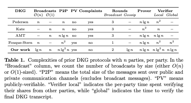
Note that PV, public verifiability, is slightly different than our requirement of verifiability: public verifiability means that any non-participating observer must be able to verify the correct execution of the DKG.
Of the schemes listed, Fouque-Stern has the lowest round complexity, however
the scheme uses Pallier which is not compatible with our encryption scheme.
The scheme described in that paper uses pairings, and thus is also not
compatible with our scheme. In addition, O(n*log*n) communication complexity
is not important for our scheme, since our vote extensions already require
n^2 communication.
In addition to these schemes, ETHDKG is in use by Anoma and Osmosis in Ferveo. However, this scheme is also not applicable to our threshold encryption scheme as it is based on pairings rather than a discrete log DKG.
FROST
Komlo and Goldberg introduced FROST: Flexible Round-Optimized Schnorr
Threshold Signatures. FROST contains a DKG which is a slightly modified
version of Pedersen’s DKG, modified to protect against rogue-key attacks. FROST
DKG operates on any prime order group where Decisional Diffie-Hellman is
difficult, and thus is compatible with decaf377.
Verifiability
FROST DKG fulfills the requirement of verifiability and security under rogue-key attacks. FROST DKG achieves this by slightly modifying Pedersen’s DKG to include a proof of knowledge of each participant’s secret in the first round of communication.
Robustness
FROST DKG trades off simplicity and efficiency in favor of robustness. A
single participant can cause the DKG to abort by contributing an invalid share
or by refusing to produce a key share. Gennaro, Jarecki, Krawczyk, and Tal
Rabin presented an alternative instantiation of Pedersen’s DKG, which
can tolerate up to n-t invalid or missing shares. This is accomplished by
adding an additional complaint round, where participants can publish evidence
of a participant’s invalid contribution and disqualify them from the DKG. A
similar strategy could be added to FROST DKG to adapt it to be robust.
Round Complexity
By including an additional round for relaying complaints from each participant to each counterparty, the round complexity of our DKG rises to 3 rounds.
ABCI++ Implementation
A prerequisite for implementing any DKG scheme in Penumbra is ABCI++, the extension to Tendermint which adds additional hooks to the Tendermint state machine interface, most importantly vote extensions.
Implementing FROST DKG with ABCI++ can be done naively by placing each round of communication in the Vote Extensions phase of ABCI++. This gives an upper bound on the delay between the start of a new epoch and the completion of the DKG as 3 blocks: 1 block per vote extension communication round.
This could potentially be pipelined by including each participant’s commitments for the next epoch (the commitments from FROST) in the block data at one of the last blocks of the previous epoch. Round 2 of FROST could occur during the vote extensions phase of the epoch transition block.
NOTE: FROST requires private communication channels for round 2, thus we
must assign validators encryption keys, perform key agreement, and encrypt
round 2 communications before placing them in the vote extension. This can be
accomplished using ECDH with decaf377, and an AEAD cipher (though
authentication is not strictly required, since vote extensions are signed).
TODO:
[] concrete robust FROST implementation
Homomorphic Threshold Encryption
The core of the flow encryption system requires a partially homomorphic encryption scheme, which allows for users to publish transactions that contain encrypted values. These encrypted values are then aggregated, using the homomorphism, by validators. The aggregate value (the “batched flow”) is then decrypted using the threshold decryption scheme described here.
Desired Properties
For our threshold encryption scheme, we require three important properties:
- Homomorphism: we must be able to operate over ciphertexts, by combining balance commitments from many participants into a batched value.
- Verifiability: we must be able to verify that a given value was encrypted correctly to a given ciphertext
- Robustness: up to validators must be permitted to either fail to provide a decryption share or provide in invalid decryption share.
Concrete Instantiation: Homomorphic ElGamal
Setup
Compute a lookup table for every by setting
where is the basepoint of decaf377.
Store for later use in value decryption.
Value Encryption
                                  ┌───────────────────┐
                                  │DKG Public Key (D) │
                                  │                   │
                                  └───────────────────┘
                                            │
                                  ┌─────────▼─────────┐    ┌──────────────┐
                                  │                   │    │     v_e      │
                                  │                   │    │  (encrypted  │
                                  │                   │    │    value)    │
                  ┌──────────┐    │ElGamal Encryption │    │ ┌──────────┐ │
               ┌─▶│v_0 (u16) │────▶   D: DKG Pubkey   ├────┼▶│   c_0    │ │
               │  └──────────┘    │     M = v_i*G     │    │ └──────────┘ │
               │  ┌──────────┐    │     e <- F_q      │    │ ┌──────────┐ │
┌────────────┐ ├─▶│v_1 (u16) │────▶ c_i = (e*G, M+eD) ├────┼▶│   c_1    │ │
│            │ │  └──────────┘    │                   │    │ └──────────┘ │
│v [0, 2^64) │─┤  ┌──────────┐    │                   │    │ ┌──────────┐ │
│            │ ├─▶│v_2 (u16) │────▶ Correctness Proof ├────┼▶│   c_2    │ │
└────────────┘ │  └──────────┘    │         σ         │    │ └──────────┘ │
               │  ┌──────────┐    │                   │    │ ┌──────────┐ │
               └─▶│v_3 (u16) │────▶                   ├────┼▶│   c_3    │ │
                  └──────────┘    │                   │    │ └──────────┘ │
                                  │                   │    │              │
                                  │                   │    │              │
                                  └───────────────────┘    └──────────────┘
                                            │
                                            │           ┌────────────────────────┐
                                            └──────────▶│proofs σ_ci = (r, s, t) │
                                                        └────────────────────────┘
A value is given by an unsigned 64-bit integer . Split into four 16-bit limbs
with .
Then, perform ElGamal encryption to form the ciphertext by taking (for each )
Where is the basepoint generator for decaf377, is the
large prime-order scalar field for decaf377, and is the public key output
from DKG.
Next, compute a proof of correctness of the ElGamal encryption by executing the following sigma protocol:
The proof is then . The encryption of value is given as .
Upon receiving an encrypted value with proofs , a validator or validating full node should verify each proof by checking
Considering the value invalid if the proof fails to verify.
This protocol proves, in NIZK, the relation
Showing that the ciphertext is an actual encryption of for the DKG pubkey , and using the hash transcript to bind the proof of knowledge of to each .
Each ciphertext is two group elements, accompanied by a proof
which is three scalars. decaf377 group elements and scalars
are encoded as 32-byte values, thus every encrypted value combined with
its proof is = 640 bytes.
Value Aggregation
                          n (batch size)
┌ ─ ─ ─ ─ ─ ─ ─ ─ ─ ─ ─ ─ ─ ─ ─ ─ ─ ─ ─ ─ ─ ─ ─ ─ ─ ─ ─ ─ ─ ─ ─ ┐
│┌──────────────┐   ┌──────────────┐            ┌──────────────┐│
 │              │   │              │            │              │
 │   v_{e0}     │   │    v_{e1}    │            │    v_{ek}    │
 │              │   │              │            │              │
 │ ┌──────────┐ │   │ ┌──────────┐ │            │ ┌──────────┐ │
 │ │   c_0    │ │   │ │   c_0    │ │            │ │   c_0    │ │
 │ └──────────┘ │   │ └──────────┘ │            │ └──────────┘ │
 │ ┌──────────┐ │   │ ┌──────────┐ │            │ ┌──────────┐ │
 │ │   c_1    │ │   │ │   c_1    │ │            │ │   c_1    │ │
 │ └──────────┘ │   │ └──────────┘ │            │ └──────────┘ │
 │ ┌──────────┐ │   │ ┌──────────┐ │    ...     │ ┌──────────┐ │
 │ │   c_2    │ │   │ │   c_2    │ │            │ │   c_2    │ │
 │ └──────────┘ │   │ └──────────┘ │            │ └──────────┘ │
 │ ┌──────────┐ │   │ ┌──────────┐ │            │ ┌──────────┐ │
 │ │   c_3    │ │   │ │   c_3    │ │            │ │   c_3    │ │
 │ └──────────┘ │   │ └──────────┘ │            │ └──────────┘ │
 │              │   │              │            │              │
 │              │   │              │            │              │
 └──────────────┘   └──────────────┘            └──────────────┘
         │                  │             │             │
         │                  │             │             │
         └──────────────────┴─────┬───────┴─────────────┘
                                  │             ┌──────────────┐
                                  ▼             │              │
                                ┌───┐           │   v_{agg}    │
                                │ + │───────────▶              │
                                └───┘           │ ┌──────────┐ │
                                                │ │   c_0    │ │
                                                │ └──────────┘ │
                                                │ ┌──────────┐ │
                                                │ │   c_1    │ │
                                                │ └──────────┘ │
                                                │ ┌──────────┐ │
                                                │ │   c_2    │ │
                                                │ └──────────┘ │
                                                │ ┌──────────┐ │
                                                │ │   c_3    │ │
                                                │ └──────────┘ │
                                                │              │
                                                │              │
                                                └──────────────┘
To batch flows, we must use the homomorphic property of ElGamal ciphertexts. Aggregation should be done component-wise, that is, on each limb of the ciphertext (). To aggregate a given , simply add each limb:
This holds due to the homomorphic property of ElGamal ciphertexts.
The block producer aggregates every , producing a public transcript of the aggregation. The transcript can then be publicly validated by any validator or full node by adding together each in the transcript and verifying that the correct was committed by the block producer.
Value Decryption
┌──────────────┐
│     v_e      │
│  (encrypted  │
│    value)    │
│ ┌──────────┐ │     ┌─────────────────────────┐
│ │   c_0    │─┼────▶│                         │    ┌─────────────────────────────────┐
│ └──────────┘ │     │                         │    │       Gossip (ABCI++ Vote       │
│ ┌──────────┐ │     │                         │    │           Extensions)           │
│ │   c_1    │─┼────▶│Decryption Shares + Proof│    │                                 │
│ └──────────┘ │     │                         │    │        verify share proof       │
│ ┌──────────┐ │     │  s_{pi} = d_{p}c_{i0}   │───▶│          σ_pi for s_pi          │
│ │   c_2    │─┼────▶│   σ_{pi} = (r, α, γ)    │    │                                 │
│ └──────────┘ │     │                         │    │      d = sum(s_pi*λ_{0,i})      │
│ ┌──────────┐ │     │                         │    │        v_mi = -d + c_{i1}       │
│ │   c_3    │─┼────▶│                         │    │                                 │
│ └──────────┘ │     └─────────────────────────┘    └─────────────────────────────────┘
│              │                                                     │    ┌───────┐
│              │                                                    ┌┘    │  LUT  │
└──────────────┘                                                    │     └───┬───┘
                   ┌─────────────────────────┐       ┌──────────────▼─────────▼────────┐
                   │                         │       │       Reverse dLog Lookup       │
                   │ Reconstruct from Limbs  │       │                                 │
                   │                         │◀──────│v_q = [LUT[v_mi], ..., LUT[v_mn]]│
                   │                         │       │                                 │
                   └─────────────────────────┘       └─────────────────────────────────┘
                                │
                                ▼
                           ┌─────────┐
                           │         │
                           │v (u128) │
                           │         │
                           └─────────┘
To decrypt the aggregate , take each ciphertext component and perform threshold ElGamal decryption using the participant’s DKG private key share to produce decryption share :
Next, each participant must compute a proof that their decryption share is well formed relative to the commitment to their secret share . This is accomplished by adopting the Chaum-Pedersen sigma protocol for proving DH-triples.
With , , and as inputs, each participant computes their proof by taking
The proof is the tuple .
Every participant then broadcasts their proof of knowledge along with their decryption share to every other participant.
After receiving from each participant, each participant verifies that is valid by checking
and aborting if verification fails. (TODO: should we ignore this participant’s share, or report/slash them?)
This protocol is the Chaum-Pedersen sigma protocol which here proves the relation
Showing that the validator’s decryption share is correctly formed for their key share which was committed to during DKG.
Now each participant can sum their received and validated decryption shares by taking
where is the lagrange coefficient (for x=0) at , defined by
where is the set of all participant indices.
Then, compute the resulting decryption by taking
Now we have the output . Each is a decaf377 group
element. Use our lookup table from the setup phase to transform each
value to its discrete log relative to the basepoint: Now
we have the decrypted value
where each is bounded in .
To recombine the value, iterate over each , packing each into a u16 value , performing carries if necessary. This yields the final value
This value is bounded by , assuming that the coefficients in the previous step were correctly bounded.
Note
On verifiability, this scheme must include some snark proof that coefficients were correctly created from input values. This can be accomplished by providing a SNARK proof that accompanies each value. It may also be desirable to SNARK the sigma protocol given in the value encryption phase in order to save on chain space.
Acknowledgements
Thanks to samczsun for his discussion and review of this spec, and for finding a flaw with an earlier instantiation of the encryption proof.
TODO: end-to-end complexity analysis (number of scalar mults per block, LUT size, etc)
Flow Encryption and Consensus
Flow encryption is marked for the next version of the protocol. The documentation will be expanded to include detailed information on flow encryption and its implementation, reflecting the ongoing enhancements in the core protocol.
Groth16 Recap
In this chapter, we’ll be looking at the internals of how Groth16’s CRS works, so it might be useful to very briefly describe how the system works. For another succinct resource on Groth16, see Kurt Pan’s Notes.
Constraint System
We work over a circuit taking inputs, which we write as . There is an index such that the are the public inputs, and the are the private inputs.
The constraints of our circuit are encoded as a list of polynomials of degree , along with a polynomial , of degree . The inputs satisfy the circuit when the following equation holds: (Note that saying that is equivalent to saying that there exists an , of degree at most , such that ).
The goal of a proof is to prove knowledge of the satisfying these constraints, without revealing information about what their values might be.
CRS
The CRS involves generating private parameters, and then performing some calculations to derive public elements, which are then used for creating and verifying proofs. It’s important that these private parameters are destroyed after being used to derive the public parameters.
As a shorthand, we define the following polynomial: which gets used many times in the CRS itself.
The private parameters consist of randomly sampled scalars:
The public parameters are then derived from these private ones, producing the following list of elements:
(Note that given for up to a given degree , we can then compute , for any polynomial of degree up to , since this element is a linear combination of these monomial elements. We write to denote this process.)
Proving and Verifying
Next we describe the proving and verification equations:
Proving
A proof consists of three group elements: , and .
The proof requires the generation of two fresh random scalars and , which are then used to compute the following elements:
Finally, the proof is returned as .
Verification
Given a proof , verification checks:
Modified CRS
BGM17 (Section 6) proposed a slightly modified CRS, adding extra elements, in order to simplify the setup ceremony. They also proved that adding these elements did not affect the security (specifically, knowledge soundness) of the scheme.
The CRS becomes:
The main change is that has been removed, and that we now have access to higher degrees of in , along with direct access to and .
Discrete Logarithm Proofs
One gadget we’ll need is a way to have ZK proofs for the following relation: (with kept secret).
In other words, one needs to prove knowledge of the discrete logarithm of with regards to .
The notation we’ll use here is for generating a proof (with some arbitrary context string ), using the public statement and the witness , as well as: for verifying that proof, using the same context and statement.
The proof should fail to verify if the context or statement don’t match, or if the proof wasn’t produced correctly, of course.
How They Work
(You can safely skip this part, if you don’t actually need to know how they work).
These are standard Maurer / Schnorr-esque proofs, making use of a hash function modelled as a random oracle.
Proving
Verification
Contributions
In this section, we describe the contributions that make up a setup ceremony in more detail. We describe:
- the high level idea behind the ceremony,
- what contributions look like, and how to check their correctness,
- how to check the correctness of the setup as a whole.
High Level Overview
We break the CRS described previously into two parts:
First, we have:
Second, we have:
We split the ceremony into two phases, to calculate the first and second part of the CRS, respectively. The general idea in each ceremony is that the secret values of interest (e.g. etc.) are shared multiplicatively, as , with each party having one of the shares. Because of this structure, given the current value of the CRS elements in a given phase, it’s possible for a new party to add their contribution. For example, in the first phase, one can multiply each element by some combination , depending on the element, to get a new CRS element.
Each contribution will come with a proof of knowledge for the new secret values contributed, which can also partially attest to how these secret values were used. However, this is not enough to guarantee that the resulting elements are a valid CRS: for this, we have a consistency check allowing us to check that the elements in a given phase have the correct internal structure.
Each party can thus contribute one after the other, until enough contributions have been gathered through that phase.
In order to link phase 1 and phase 2, we use the fact that with , the CRS elements of phase 2 are linear combinations of those in phase 1. If we consider , with up to , the largest monomial we’ll find is , since has degree at most . In the first phase, we calculated these powers of , and so can calculate these values by linear combination. We can do the same for: since we have access to and for sufficiently high degrees.
Phase 1
Assuming we have the CRS elements of phase 1, a contribution involves fresh random scalars , and produces the following elements:
Additionally, a contribution includes three proofs:
Checking Correctness
Given purported CRS elements:
We can check their validity by ensuring the following checks hold:
- Check that (the identity element in the respective groups).
- Check that .
- Check that .
- Check that .
- Check that .
- Check that .
Checking Linkedness
To check that CRS elements build off a prior CRS , one checks the included discrete logarithm proofs , via:
Phase 2
Assuming we have the CRS elements of phase 2, a contribution involves a fresh random scalar , and produces the following elements:
Additionally, a contribution includes a proof:
Checking Correctness
Assume that the elements and are known.
Then, given purported CRS elements:
We can check their validity by ensuring the following checks hold:
- Check that (the identity element in the respective groups).
- Check that .
- Check that .
- Check that .
Checking Linkedness
To check that CRS elements build off a prior CRS , one checks the included discrete logarithm proof , via:
Batched Pairing Checks
Very often, we need to check equations of the form: (this would also work if the right-hand side is of the form , and vice versa).
This equation is equivalent to checking: If you pick random scalars from a set , then except with probability , this is equivalent to checking: By the homomorphic properties of a pairing, this is the same as:
Instead of checking pairings, we can instead perform MSMs of size , and then pairings, which is more performant.
Addresses and Keys
The key hierarchy is a modification of the design in Zcash Sapling. The main
differences are that it is designed for use with BLS12-377 rather than
BLS12-381, that it also uses Poseidon1 as a hash and PRF, decaf377 as the embedded
group, and that it includes support for fuzzy message
detection.
All key material within a particular spend authority - an account - is ultimately derived from a single root secret. The internal key components and their derivations are described in the following sections:
- Spending Keys describes derivation of the spending key from the root key material;
- Viewing Keys describes derivation of the full, incoming, and outgoing viewing keys;
- Addresses and Detection Keys describes derivation of multiple, publicly unlinkable addresses for a single account, each with their own detection key.
The diagram in the Overview section describes the key hierarchy from an external, functional point of view. Here, we zoom in to the internal key components, whose relations are depicted in the following diagram. Each internal key component is represented with a box; arrows depict key derivation steps, and diamond boxes represent key derivation steps that combine multiple components.
flowchart BT
    subgraph Address
        direction TB;
        d2[d];
        pk_d;
        ck_d;
    end;
    subgraph DTK[Detection Key]
        dtk_d;
    end;
    subgraph IVK[Incoming\nViewing Key]
        ivk;
        dk;
    end;
    subgraph OVK[Outgoing\nViewing Key]
        ovk;
    end;
    subgraph FVK[Full Viewing Key]
        ak;
        nk;
    end;
    subgraph SK[Spending Key]
        direction LR;
        ask;
        spend_key_bytes;
    end;

    BIP44(BIP44 Seed Phrase) --> spend_key_bytes;
    BIP39(Legacy Raw BIP39) --> spend_key_bytes;

    spend_key_bytes --> ask;
    spend_key_bytes --> nk;

    ask --> ak;

    ak & nk --> fvk_blake{ };
    ak & nk --> fvk_poseidon{ };
    fvk_blake --> ovk & dk;
    fvk_poseidon --> ivk;

    index(address index);
    d1[d];

    d1 --- d2;

    index --> aes{ };
    dk ---> aes{ };
    aes --> d1;

    d1 & ivk --> scmul_ivk{ };
    scmul_ivk --> pk_d;

    d1 & ivk --> dtk_blake{ };
    dtk_blake --> dtk_d;
    dtk_d --> ck_d;
In general, the Poseidon hash function is used in places where hashing needs to be done in-circuit, for example, when hashing new commitments into the state commitment tree. Elsewhere in the protocol, we use BLAKE2b-512 e.g. in the derivation of the spend authorization key, which is not done in-circuit.
Spending Keys
A BIP39 12- or 24-word seed phrase can be used to derive one or more spend authorities.
Legacy Raw BIP39 Derivation
Prior to Testnet 62, from this mnemonic seed phrase, spend seeds were derived
using PBKDF2 with:
HMAC-SHA512as the PRF and an iteration count of 2048 (following BIP39)- the seed phrase used as the password
mnemonicconcatenated with a passphrase used as the salt, where the default spend authority was derived using the saltmnemonic0.
Default BIP44 Derivation
Beginning in Testnet 62, from the mnemonic seed phrase, spend seeds were derived
as described in BIP44. The BIP44 specification describes an organizational
hierarchy allowing a user to remember a single seed phrase for multiple
cryptocurrencies.
The BIP44 path for Penumbra consists of:
m / purpose' / coin_type' / wallet_id'
m represents the master node and is derived from the spend seed as described in
BIP32 in section “Master key generation”.
The purpose field is a constant set to 44' to denote that BIP44 is being used.
Penumbra’s registered coin_type is defined in SLIP-0044:
- Coin type:
6532 - Path component
coin_type' = 0x80001984
The default wallet ID is set to 0. A typical use case for Penumbra will involve generating the single default wallet, and then using multiple Penumbra accounts within that wallet which share a single viewing key.
The BIP44 path is used with the seed phrase to derive the spend seed for use
in Penumbra following the child key derivation specified in BIP32.
The root key material for a particular spend authority is the 32-byte
spend_key_bytes derived as above from the seed phrase. The spend_key_bytes value is used to derive
- , the spend authorization key, and
- , the nullifier key,
as follows. Define prf_expand(label, key, input) as BLAKE2b-512 with
personalization label, key key, and input input. Define
from_le_bytes(bytes) as the function that interprets its input bytes as an
integer in little-endian order. Then
ask = from_le_bytes(prf_expand("Penumbra_ExpndSd", spend_key_bytes, 0)) mod r
nk  = from_le_bytes(prf_expand("Penumbra_ExpndSd", spend_key_bytes, 1)) mod q
The spending key consists of spend_key_bytes and ask. (Since ask is
derived from spend_key_bytes, only the spend_key_bytes need to be stored,
but the ask is considered part of the spending key). When using a hardware
wallet or similar custody mechanism, the spending key remains on the device.
The spend authorization key is used as a decaf377-rdsa signing
key.1 The corresponding verification key is the spend verification key
. The spend verification key and
the nullifier key are used to create the full viewing key
described in the next section.
Note that it is technically possible for the derived or to be , but this happens with probability approximately , so we ignore this case, as, borrowing phrasing from Adam Langley, it happens significantly less often than malfunctions in the CPU instructions we’d use to check it.
Viewing Keys
Each spending key has a corresponding collection of viewing keys, which represent different subsets of capability around creating and viewing transactions:
- the full viewing key represents all capability except for spend authorization, including viewing all incoming and outgoing transactions and creating proofs;
- the incoming viewing key represents the capability to scan the blockchain for incoming transactions;
- the outgoing viewing key represents the capability to recover information about sent transactions.
Full Viewing Keys
The full viewing key consists of two components:
- , the spend verification key, a
decaf377-rdsaverification key; - , the nullifier key.
Their derivation is described in the previous section.
The spend verification key is used (indirectly) to verify spend authorizations. Using it directly would allow spends signed by the same key to be linkable to each other, so instead, each spend is signed by a randomization of the spend authorization key, and the proof statement includes a proof that the verification key provided in the spend description is a randomization of the (secret) spend verification key.
The nullifier key is used to derive the nullifier of a note sent to a particular user. Nullifiers are used for double-spend protection and so must be bound to the note contents, but it’s important that nullifiers cannot be derived solely from the contents of a note, so that the sender of a note cannot learn when the recipient spent it.
The full viewing key can be used to create transaction proofs, as well as to view all activity related to its account. The hash of a full viewing key is referred to as an Account ID and is derived as follows.
Define
poseidon_hash_2(label, x1, x2) to be rate-2 Poseidon hashing of inputs x1,
x2 with the capacity initialized to the domain separator label. Define
from_le_bytes(bytes) as the function that interprets its input bytes as an
integer in little-endian order. Define
element.to_le_bytes() as the function that encodes an input element in
little-endian byte order. Define decaf377_s(element) as the function
that produces the -value used to encode the provided decaf377 element.
Then
hash_output = poseidon_hash_2(from_le_bytes(b"Penumbra_HashFVK"), nk, decaf377_s(ak))
wallet_id = hash_output.to_le_bytes()[0:32]
i.e. we take the 32-bytes of the hash output as the account ID.
Incoming and Outgoing Viewing Keys
The incoming viewing key consists of two components:
- , the diversifier key, and
- , the incoming viewing key (component)1.
The diversifier key is used to derive diversifiers, which allow a single spend authority to have multiple, publicly unlinkable diversified addresses, as described in the next section. The incoming viewing key is used to scan the chain for transactions sent to every diversified address simultaneously.
The outgoing viewing key consists of one component:
- , the outgoing viewing key (component).
These components are derived as follows.
The and are not intended to be derived in a
circuit. Define prf_expand(label, key, input) as BLAKE2b-512 with
personalization label, key key, and input input. Define
to_le_bytes(input) as the function that encodes an input integer in
little-endian byte order. Define decaf377_encode(element) as the function
that produces the canonical encoding of a decaf377 element. Then
ovk  = prf_expand(b"Penumbra_DeriOVK", to_le_bytes(nk), decaf377_encode(ak))[0..32]
dk = prf_expand(b"Penumbra_DerivDK", to_le_bytes(nk), decaf377_encode(ak))[0..16]
The is intended to be derived in a circuit. Then
ivk = poseidon_hash_2(from_le_bytes(b"penumbra.derive.ivk"), nk, decaf377_s(ak)) mod r
i.e., we treat the Poseidon output (an element) as an integer, and reduce it modulo to get an element of .
In general, we refer to the combination of and as the “incoming viewing key” and the component just as , using the modifier “component” in case of ambiguity.
Addresses and Detection Keys
Rather than having a single address for each spending authority, Penumbra allows the creation of many different publicly unlinkable diversified addresses. An incoming viewing key can scan transactions to every diversified address simultaneously, so there is no per-address scanning cost. In addition, Penumbra attaches a detection key to each address, allowing a user to outsource probabilistic transaction detection to a relatively untrusted third-party scanning service.
Privacy Implications
While diversified addresses are described as publicly unlinkable, a detection entity given multiple detection keys can empirically link the corresponding diversified addresses via the clue keys contained within them. This is because the detection entity, by reporting detected transactions to the same user, empirically knows that the detection keys are linked. If the detection entity observes two addresses belonging to the user, they can link them because the clue key appears in each address and is derived solely from the detection key.
In a simplified scenario, a user with diversified addresses and gives the associated detection keys and to the detection entity. The detection entity detects relevant transactions using the clue keys and , and reports the detected transactions for and back to the user. The detection entity can naively observe that transactions related to and are reported back to the same user, and therefore the addresses linked to these detection keys belong to the same user. There’s a notion of linkability here since the diversified addresses can be linked by the detection entity through the detection keys, from which the clue keys are derived.
To mitigate the linkability of diversified addresses when using detection keys, a user should consider using multiple third parties: distribute detection keys to different detection entities instead of a single one, reducing the risk that any single entity has enough keys to link diversified addresses.
Diversifiers
Addresses are parameterized by diversifiers, 16-byte tags used to derive up to distinct addresses for each spending authority. The diversifier is included in the address, so it should be uniformly random. To ensure this, diversifiers are indexed by a address index ; the -th diversifier is the encryption of using AES with the diversifier key .1
Each diversifier is used to generate a diversified basepoint as
where
performs hash-to-group for decaf377 as follows: first, apply BLAKE2b-512
with personalization b"Penumbra_Divrsfy" to the input, then, interpret the
64-byte output as an integer in little-endian byte order and reduce it modulo
, and finally, use the resulting element as input to the
decaf377 CDH map-to-group method.
Detection Keys
Each address has an associated detection key, allowing the creator of the address to delegate a probabilistic detection capability to a third-party scanning service.
The detection key consists of one component,
- , the detection key (component)2,
derived as follows. Define prf_expand(label, key, input) as BLAKE2b-512 with
personalization label, key key, and input input. Define
from_le_bytes(bytes) as the function that interprets its input bytes as an
integer in little-endian order, and to_le_bytes as the function that encodes
an integer to little-endian bytes. Then
dtk_d = from_le_bytes(prf_expand(b"PenumbraExpndFMD", to_le_bytes(ivk), d))
Addresses
Each payment address has three components:
- the diversifier ;
- the transmission key , a
decaf377element; - the clue key , a
decaf377element.
The diversifier is derived from an address index as described above. The diversifier with index is the default diversifier, and corresponds to the default payment address.
The transmission key is derived as , where is the diversified basepoint.
The clue key is is derived as , where is the conventional decaf377 basepoint.
Address Encodings
The raw binary encoding of a payment address is the 80-byte string d || pk_d || ck_d. We then apply the F4Jumble algorithm to
this string. This mitigates attacks where an attacker replaces a valid
address with one derived from an attacker controlled key that encodes to an
address with a subset of characters that collide with the target valid address.
For example, an attacker may try to generate an address with the first
characters matching the target address. See ZIP316 for more on this
scenario as well as F4Jumble, which is a 4-round Feistel construction.
This jumbled string is then encoded with Bech32m with the following human-readable prefixes:
penumbrafor mainnet, andpenumbra_tnXYZ_for testnets, where XYZ is the current testnet number padded to three decimal places.
Short Address Form
Addresses can be displayed in a short form. A short form of length bits (excludes the human-readable prefix) is recommended to mitigate address replacement attacks. The attacker’s goal is to find a partially colliding prefix for any of addresses they have targeted.
Untargeted attack
In an untargeted attack, the attacker wants to find two different addresses that have a colliding short form of length bits.
A collision is found in steps due to the birthday bound, where is the number of bits of the prefix.
Thus we’d need to double the length to provide a desired security level of bits.
This is equivalent to characters of the Bech32m address, excluding the human-readable prefix. Thus for a targeted security level of 80 bits, we’d need a prefix length of 160 bits, which corresponds to 32 characters of the Bech32m address, excluding the human-readable prefix.
The short form is not intended to mitigate this attack.
Single-target attack
In a targeted attack, the attacker’s goal is to find one address that collides with a target prefix of length bits.
Here the birthday bound does not apply. To find a colliding prefix of the first M bits, they need to search addresses.
The short form is intended to mitigate this attack.
Multi-target attack
In a multi-target attack, the attacker’s goal is to be able to generate one address that collides with the short form of 1 of different addresses.
They are searching for a collision between the following two sets:
- set of the short forms of the targeted addresses, which has size elements, and each element has length bits.
- set of the short forms of all addresses, which has size elements.
If the attacker has a target set of addresses, she can find a collision after steps. Thus for a prefix length of bits, we get bits of security. For a targeted security level of 80 bits and a target set of size , we need a prefix length of 120 bits, which corresponds to 24 characters of the Bech32m address, excluding the human-readable prefix and separator.
The short form is intended to mitigate this attack.
This convention is not enforced by the protocol; client software could in principle construct diversifiers in another way, although deviating from this mechanism risks compromising privacy.
As in the previous section, we use the modifier “component” to distinguish between the internal key component and the external, opaque key.
Transaction Cryptography
This section describes the transaction-level cryptography that is used in Penumbra actions to symmetrically encrypt and decrypt swaps, notes, and memos.
For the symmetric encryption described in this section, we use ChaCha20-Poly1305 (RFC-8439).
It is security-critical that (key, nonce) pairs are not reused. We do this by either:
- deriving per-action keys from ephemeral shared secrets using a fixed nonce (used for notes and memo keys),
- deriving per-action keys from the outgoing viewing key using a fixed nonce (used for swaps).
We use each key at maximum once with a given nonce. We describe the nonces and keys below.
Nonces
We use a different nonce to encrypt each type of item using the following [u8; 12] arrays:
- Notes:
[0, 0, 0, 0, 0, 0, 0, 0, 0, 0, 0, 0] - Memos:
[1, 0, 0, 0, 0, 0, 0, 0, 0, 0, 0, 0] - Swaps:
[2, 0, 0, 0, 0, 0, 0, 0, 0, 0, 0, 0] - Memo keys:
[3, 0, 0, 0, 0, 0, 0, 0, 0, 0, 0, 0]
Keys
We have several keys involved in transaction-level symmetric cryptography:
- A shared secret derived between sender and recipient,
- A per-action payload key used to encrypt a single note or memo key (one of each type). It is derived from the shared secret. It is used for a single action.
- A per-action swap payload key used to encrypt a single swap. It is derived from the outgoing viewing key. It is used for a single action.
- A random payload key used to encrypt a memo. It is generated randomly and is shared between all actions in a given transaction.
- An outgoing cipher key used to encrypt key material (the shared secret) to enable the sender to later decrypt an outgoing swap, note, or memo.
- An OVK wrapped key - this is the shared secret encrypted using the sender’s outgoing cipher key. A sender can later use this field to recover the shared secret they used when encrypting the note, swap, or memo to a recipient.
- A wrapped memo key - this is the memo key encrypted using the per-action payload key. The memo key used for a (per-transaction) memo is shared between all outputs in that transaction. The wrapped key is encrypted to their per-action payload key.
In the rest of this section, we describe how each key is derived.
Shared Secret
A shared secret shared_secret is derived between sender and recipient by performing Diffie-Hellman
key exchange between:
- an ephemeral secret () and the diversified transmission key of the recipient (described in more detail in the Addresses section),
- the ephemeral public key (where ), provided as a public field in the action, and the recipient’s incoming viewing key .
This allows both sender and recipient to generate the shared secret based on the keys they possess.
Per-action Payload Key: Notes and Memo Keys
The symmetric per-action payload key is a 32-byte key derived from the shared_secret, the and
personalization string “Penumbra_Payload”:
action_payload_key = BLAKE2b-512("Penumbra_Payload", shared_secret, epk)
This symmetric key is then used with the nonces specified above to encrypt a memo key or note. It must not be used to encrypt two items of the same type.
Per-action Payload Key: Swaps
The symmetric per-action payload key is a 32-byte key derived from the outgoing viewing
key ovk, the swap commitment cm, and personalization string “Penumbra_Payswap”:
action_payload_key = BLAKE2b-512("Penumbra_Payswap", ovk, cm)
This symmetric key is used with the nonces specified above to encrypt a swap only. We use the outgoing viewing key for swaps since third parties cannot create swaps for a given recipient, i.e. the user only sends swaps to themselves.
Random Payload Key: Memo
The random payload key is a 32-byte key generated randomly. This symmetric key is used with the nonces specified above to encrypt memos only. This key is provided to all output actions in a given transaction, as all outputs should be able to decrypt the per-transaction memo.
Outgoing Cipher Key
The symmetric outgoing cipher key is a 32-byte key derived from the sender’s outgoing viewing key , the balance commitment , the note commitment , the ephemeral public key , and personalization string “Penumbra_OutCiph”:
outgoing_cipher_key = BLAKE2b-512("Penumbra_OutCiph", ovk, cv, cm, epk)
All inputs except the outgoing viewing key are public. The intention of the outgoing cipher key is to enable the sender to view their outgoing transactions using only their outgoing viewing key. The outgoing cipher key is used to encrypt data that they will need to later reconstruct any outgoing transaction details.
OVK Wrapped Key
To decrypt outgoing notes or memo keys, the sender needs to store the shared secret encrypted
using the outgoing cipher key described above. This encrypted data,
48-bytes in length (32 bytes plus 16 bytes for
authentication) we call the OVK wrapped key and is saved on OutputBody.
The sender later scanning the chain can:
- Derive the outgoing cipher key as described above using their outgoing viewing key and public fields.
- Decrypt the OVK wrapped key.
- Derive the per-action payload key and use it to decrypt the corresponding memo or note.
Wrapped Memo Key
The wrapped memo key is 48 bytes in length (32 bytes plus 16 bytes for authentication).
It is saved on the OutputBody and is encrypted using the per-action payload key.
State Commitment Tree
Penumbra makes an explicit separation between two different kinds of state:
- Public shared state, recorded on-chain in a key-value store;
- Private per-user state, recorded on end-user devices and only committed to on-chain.
Public state is global and mutable, like other blockchains (akin to an “account model”). Transactions modify the public state as they execute. Private state is recorded in immutable, composable state fragments (akin to a “UTXO model”). Transactions privately consume existing state fragments, compose them to privately create new state fragments, and use zero-knowledge proofs to certify that the new fragments were created according to the rules of the protocol.
The state commitment tree component manages commitments to private state fragments. Nodes maintain two data structures, each responsible for one side of state management:
- The state commitment tree ingests and records new state commitments as transactions produce new state fragments;
- The nullifier set is responsible for nullifying existing state commitments as transactions consume state fragments.
To establish that a state fragment was previously validated by the chain, a client forms a ZK proof that the commitment to that state fragment is included in the state commitment tree. This allows private execution to reference prior state fragments, without revealing which specific state fragment is referenced.
Private execution involves a role reversal relative to the conventional use of Merkle trees in blockchains, because it is the client that makes a proof to the full node, rather than the other way around. This means that every client must synchronize a local instance of the state commitment tree, in order to have the data required to form proofs. Penumbra’s state commitment tree is instantiated using the tiered commitment tree (TCT), an append-only, ZK-friendly Merkle tree designed primarily for efficient, filterable synchronization. We use the term SCT to refer to the part of the protocol that manages state commitments and TCT to refer to the specific Merkle tree construction used to instantiate it. The TCT is described in the Tiered Commitment Tree section.
Establishing that a state fragment was previously validated by the chain is not enough, however. Clients also need to establish that the state fragments their transaction consumes have not already been consumed by another transaction, to prevent double-spend attacks.
This is accomplished by the use of nullifiers, described in detail in the Nullifiers section. Each state commitment has an associated nullifier. Transactions reveal the nullifiers of state fragments they consume, and the chain checks that they have not been previously revealed. Nullifiers can only be derived by the actor with authority over the state fragment, so the creation of a state fragment (revealing its state commitment) and the consumption of that state fragment (revealing its nullifier) are publicly unlinkable. In practice, the nullifier set is stored in the public state using the Jellyfish Merkle Tree (JMT).
Tiered Commitment Tree
The Penumbra protocol’s state commitment tree (SCT) stores cryptographic commitments to shielded state, such as note and swap commitments. The SCT is instantiated using the tiered commitment tree (TCT) data structure, an append-only, ZK-friendly Merkle tree. The unique features of the TCT are that it is:
-
Quaternary: Each node of the tiered commitment tree has four children. This means that the tree can be much shallower while having the same amount of capacity for leaves, which reduces the number of hash operations required for each insertion. The academic research surrounding the Poseidon hash recommends a quaternary tree specifically for its balance between proof depth and proof size: a binary tree means too many expensive hash operations, whereas an octal tree means too large proofs.
-
Sparse: A client’s version of the tree need only represent the state commitments pertinent to that client’s state, with all other “forgotten” commitments and internal hashes related to them pruned to a single summary hash.
-
Semi-Lazy: The internal hashes along the frontier of the tree are only computed on demand when providing a proof of inclusion or computing the root hash of the tree, which means a theoretical performance boost of (amortized) 12x during scanning.
-
Tiered: the structure of the tree is actually a triply-nested tree-of-trees-of-trees. The global, top-level tree contains at its leaves up to 65,536 epoch trees, each of which contains at its own leaves up to 65,536 block trees, each of which contains at its own leaves up to 65,536 note commitments. It is this structure that enables a client to avoid ever performing the hashes to insert the state commitments in blocks or epochs when it knows it didn’t receive any notes or swaps. When a client detects that an entire block, or an entire epoch, contained nothing of interest for it, it doesn’t need to construct that span of the commitment tree: it merely inserts the singular summary hash for that block or epoch, which is provided by the chain itself inline with the stream of blocks.
Eternity┃           ╱╲ ◀───────────── Anchor
    Tree┃          ╱││╲               = Global Tree Root
        ┃         * ** *           ╮
        ┃      *   *  *   *        │ 8 levels
        ┃   *     *    *     *     ╯
        ┃  ╱╲    ╱╲    ╱╲    ╱╲
        ┃ ╱││╲  ╱││╲  ╱││╲  ╱││╲ ◀─── Global Tree Leaf
                        ▲             = Epoch Root
                     ┌──┘
                     │
                     │
   Epoch┃           ╱╲ ◀───────────── Epoch Root
    Tree┃          ╱││╲
        ┃         * ** *           ╮
        ┃      *   *  *   *        │ 8 levels
        ┃   *     *    *     *     ╯
        ┃  ╱╲    ╱╲    ╱╲    ╱╲
        ┃ ╱││╲  ╱││╲  ╱││╲  ╱││╲ ◀─── Epoch Leaf
                 ▲                    = Block Root
                 └───┐
                     │
                     │
   Block┃           ╱╲ ◀───────────── Block Root
    Tree┃          ╱││╲
        ┃         * ** *           ╮
        ┃      *   *  *   *        │ 8 levels
        ┃   *     *    *     *     ╯
        ┃  ╱╲    ╱╲    ╱╲    ╱╲
        ┃ ╱││╲  ╱││╲  ╱││╲  ╱││╲ ◀─── Block Leaf
                                      = State Commitment
Nullifiers
Each positioned state commitment has an associated nullifier, an element. We say that a state commitment is positioned when it has been included in the state commitment tree and its position is fixed. In other words, a nullifier is not just a property of the content of a state fragment, but of a specific instance of a state fragment included in the chain state.
Nullifiers are not publicly derivable from the state fragment. Instead, each state fragment defines an associated nullifier key, also an element. The nullifier key represents the capability to derive the nullifier associated to a state fragment. When state fragments are created, their state commitment is revealed on-chain, and when they are consumed, their nullifier is revealed. These actions are unlinkable without knowledge of the nullifier key.
Nullifier Derivation
The nullifier (an element) is derived as the following output of a rate-3 Poseidon hash:
nf = hash_3(ds, (nk, cm, pos))
where the ds is a domain separator as described below, nk is the
nullifier key, cm is the state commitment, and pos is the position
of the state commitment in the state commitment tree.
Define from_le_bytes(bytes) as the function that interprets its input bytes as
an integer in little-endian order. The domain separator ds used for nullifier
derivation is computed as:
ds = from_le_bytes(BLAKE2b-512(b"penumbra.nullifier")) mod q
Nullifier Keys
Nullifiers are derived only semi-generically. While the nullifier derivation itself is generic, depending only on the nullifier key and the positioned commitment, each type of state fragment is responsible for defining how the nullifier key is linked to the content of that state fragment. Because nullifiers prevent double-spends, this linking is critical for security.
This section describes the abstract properties required for nullifier key linking, and how each type of state fragment achieves those properties.
- Uniqueness: each state fragment must have at most one nullifier key.
Uniqueness ensures that each state fragment can be nullified at most once. A state fragment without a nullifier key is unspendable; this is likely undesirable, like sending funds to a burn address, but is not prohibited by the system. If a state fragment had more than one nullifier key, it could be consumed multiple times, causing a double-spend vulnerability.
Each action that reveals nullifiers is responsible for certifying two distinct properties as part of its proof statements:
- Correct derivation of the nullifier given the nullifier key and positioned state commitment (generic across state fragment types);
- Correct linking of that nullifier key with the content of the nullified state fragment (specific to that state fragment type).
State Fragments
These are the current types of state fragment recorded by Penumbra:
Notes
The nullifier key for a note is the nullifier key component of the full viewing key for the address controlling the note.
Uniqueness: Nullifiers are unique, to prevent faerie gold attacks, as they are derived from the position in the state commitment tree which is unique.
Swaps
The nullifier key for a swap is the nullifier key component of the full viewing key for the claim address that controls the swap outputs.
Uniqueness: TODO
Assets and Values
Penumbra can record arbitrary assets. These assets either originate on Penumbra itself, or, more commonly, originate on other IBC-connected chains. To record arbitrary assets and enforce value balance between them, we draw on ideas originally proposed for Zcash and adapt them to the Cosmos context.
Asset types and asset IDs
To be precise, we define:
- an amount to be an untyped
u128quantity of some asset; - an asset ID to be an element;
- a value to be a typed quantity, i.e., an amount and an asset ID.
All asset IDs are currently computed as the hash of a denomination, an ADR001-style denomination trace uniquely identifying a cross-chain asset and its provenance, such as:
denom(native chain A asset)transfer/channelToA/denom(chain B representation of chain A asset)transfer/channelToB/transfer/channelToA/denom(chain C representation of chain B representation of chain A asset)
However, Penumbra deviates slightly from ADR001 in the definition of the asset
ID. While ADR001 defines the IBC asset ID as the SHA-256 hash of the
denomination trace, Penumbra hashes to a field element, so that asset IDs can be
more easily used inside of a zk-SNARK circuit. Specifically, define
from_le_bytes(bytes) as the function that interprets its input bytes as an
integer in little-endian order, and hash(label, input) as BLAKE2b-512 with
personalization label on input input. Then asset IDs are computed as
asset_id = from_le_bytes(hash(b"Penumbra_AssetID", asset_type)) mod q
In the future, Penumbra may have other asset IDs do not correspond to denominations, but are computed as hashes of other state data. By making the asset ID itself be a hash of extended state data, a note recording value of that type also binds to that extended data, even though it has the same size as any other note. Currently, however, all asset IDs are computed as the hashes of denomination strings.
Asset Metadata
Penumbra also supports Cosmos-style Metadata for assets. The chain maintains
an on-chain lookup table of asset IDs to asset metadata, but the on-chain
metadata is minimal and generally only includes the denomination string. Client
software is expected to be opinionated about asset metadata, supplying
definitions with symbols, logos, etc. to help users understand the assets they
hold.
Value Generators
Each asset ID has an associated value generator . The value generator is computed as , where is a hash-to-group function constructed by first applying
rate-1 Poseidon hashing with domain separator
from_le_bytes(blake2b(b"penumbra.value.generator")) and then the decaf377 CDH
map-to-group method.
Homomorphic Balance Commitments
We use the value generator associated to an asset ID to construct additively homomorphic commitments to (typed) value. To do this, we first define the blinding generator as
V_tilde = decaf377_encode_to_curve(from_le_bytes(blake2b(b"decaf377-rdsa-binding")))
The commitment to value , i.e., amount of asset , with random blinding factor , is the Pedersen commitment
These commitments are homomorphic, even for different asset types, say values and :
where and are generators of the group , and and are random blinding factors from .
Alternatively, this can be thought of as a commitment to a (sparse) vector recording the amount of every possible asset type, almost all of whose coefficients are zero.
Transaction Model
A Penumbra transaction is a bundle of actions that effect changes to the chain state, together with additional data controlling how those actions are executed or providing additional metadata. All actions in the transaction are executed together, and the transaction succeeds or fails atomically. A transaction body has four parts:
- A list of actions effecting changes to the chain state;
- A set of
TransactionParametersdescribing conditions under which the actions may be executed; - An optional set of
DetectionDatathat helps third-party servers detect transactions using Fuzzy Message Detection; - An optional
MemoCiphertextwith an encrypted memo visible only to the sender and receiver(s) of the transaction.
The Transaction Signing section describes transaction authorization.
Actions and Value Balance
The primary content of a transaction is its list of actions. Each action is executed in sequence, and effects changes to the chain state.
Crucially, each action makes a shielded contribution to the transaction’s value balance by means of a balance commitment, using the commitment scheme for asset values described in detail in the Asset Model.
Some actions, like a Spend, consume state fragments from the chain and release
value into the transaction, while others, like Output, consume value from the
transaction and record it in the state. And actions like Delegate consume one
type of value (the staking token) and release another type of value (the
delegation token).
The chain requires that transactions do not create or destroy value. To accomplish conservation of value, the binding signature proves that the transaction’s value balance, summed up over all actions, is zero. This construction works as follows. We’d like to be able to prove that a certain balance commitment is a commitment to . One way to do this would be to prove knowledge of an opening to the commitment, i.e., producing such that But this is exactly what it means to create a Schnorr signature for the verification key , because a Schnorr signature is a proof of knowledge of the signing key in the context of the message.
Therefore, we can prove that a balance commitment is a commitment to by
treating it as a decaf377-rdsa verification key and using the corresponding
signing key (the blinding factor) to sign a message. This also gives a way to
bind balance commitments to a particular context (e.g., a transaction), by using a
hash of the transaction as the message to be signed, ensuring that actions
cannot be replayed across transactions without knowledge of their contents.
The balance commitment mechanism is essential to security. It is what “glues” the validity of the local state transitions provided by each action’s proof statement into validity of the global state transition.
A complete list of actions and a summary of their effects on the chain state and the transaction’s value balance is provided in the Action Reference.
Transaction Signing
In a transparent blockchain, a signer can inspect the transaction to be signed to validate the contents are what the signer expects. However, in a shielded blockchain, the contents of the transaction are opaque. Ideally, using a private blockchain would enable a user to sign a transaction while also understanding what they are signing.
To avoid the blind signing problem, in the Penumbra protocol we allow the user
to review a description of the transaction - the TransactionPlan - prior to
signing. The TransactionPlan contains a declarative description of all details of the proposed transaction, including a plan of each action in a transparent
form, the fee specified, the chain ID, and so on. From this plan, we authorize the and build the transaction. This has the additional advantage of allowing the signer to authorize the
transaction while the computationally-intensive Zero-Knowledge
Proofs (ZKPs) are optimistically generated as part of the transaction build process.
The signing process first takes a TransactionPlan and SpendKey and returns
the AuthorizationData, essentially a bundle of signatures over
the effect hash, which can be computed directly from the plan data. You can
read more about the details of the effect hash computation below.
The building process takes the TransactionPlan, generates the proofs, and constructs a fully-
formed Transaction. This process is internally partitioned into three steps:
- Each
Actionis individually built based to its specification in theTransactionPlan. - The pre-built actions to collectively used to construct a transaction with placeholder dummy signatures, that can be filled in once the
signatures from the
AuthorizationDataare ready1. This intermediate state of the transaction without the full authorizing data is referred to as the “Unauthenticated Transaction”. - Slot the
AuthorizationDatato replace the placeholder signatures to assemble the finalTransaction.
The Penumbra protocol was designed to only require the custodian, e.g. the hardware wallet environment, to do signing, as the generation of ZKPs can be done without access to signing keys, requiring only witness data and viewing keys.
A figure showing how these pieces fit together is shown below:
╔════════════════════════╗
║         Authorization  ║
║                        ║
║┌──────────────────────┐║
║│ Spend authorization  │║
║│         key          │║    ┌───────────────────┐
║└──────────────────────┘║    │                   │
║                        ║───▶│ AuthorizationData │──┐
║                        ║    │                   │  │
║┌──────────────────────┐║    └───────────────────┘  │
║│      EffectHash      │║                           │
║└──────────────────────┘║                           │
║                        ║                           │
║                        ║                           │
╚════════════▲═══════════╝                           │
             │                                       │
             │                                       │               ┌───────────┐
 ┌───────────┴───────────┐                           │               │           │
 │                       │                           └─────────┬────▶│Transaction│
 │    TransactionPlan    │                                     |     │           │
 │                       │                                     │     └───────────┘
 └───────────┬───────────┘                                     │
             │                                                 │
             │                                                 │
             │                                                 │
 ╔═══════════▼════════════╗                                    │
 ║                Proving ║                                    │
 ║                        ║                                    │
 ║┌──────────────────────┐║                                    │
 ║│     WitnessData      │║                                    │
 ║└──────────────────────┘║   ┌──────────────────────────────┐ │
 ║                        ║   │                              │ │
 ║                        ╠──▶│ Unauthenticated Transaction  ├─┘
 ║┌──────────────────────┐║   │                              │
 ║│   Full viewing key   │║   └──────────────────────────────┘
 ║└──────────────────────┘║
 ║                        ║
 ║                        ║
 ║                        ║
 ╚════════════════════════╝
Transactions are signed used the decaf377-rdsa construction. As described briefly in that section, there are two signature domains used in Penumbra: SpendAuth signatures and Binding signatures.
SpendAuth Signatures
SpendAuth signatures are included on each Spend and DelegatorVote action
(see Multi-Asset Shielded Pool and Governance
for more details on Spend and DelegatorVote actions respectively).
The SpendAuth signatures are created using a randomized signing key and the corresponding randomized verification key provided on the action. The purpose of the randomization is to prevent linkage of verification keys across actions.
The SpendAuth signature is computed using the decaf377-rdsa Sign algorithm
where the message to be signed is the effect hash of the entire transaction
(described below), and the decaf377-rdsa domain is SpendAuth.
Effect Hash
The effect hash is computed over the effecting data of the transaction, which following the terminology used in Zcash2:
“Effecting data” is any data within a transaction that contributes to the effects of applying the transaction to the global state (results in previously-spendable coins or notes becoming spent, creates newly-spendable coins or notes, causes the root of a commitment tree to change, etc.).
The data that is not effecting data is authorizing data:
“Authorizing data” is the rest of the data within a transaction. It does not contribute to the effects of the transaction on global state, but allows those effects to take place. This data can be changed arbitrarily without resulting in a different transaction (but the changes may alter whether the transaction is allowed to be applied or not).
For example, the nullifier on a Spend is effecting data, whereas the
proofs or signatures associated with the Spend are authorizing data.
In Penumbra, the effect hash of each transaction is computed using the BLAKE2b-512 hash function. The effect hash is derived from the proto-encoding of the action - in cases where the effecting data and authorizing data are the same, or the body of the action - in cases where the effecting data and authorizing data are different. Each proto has a unique string associated with it called its Type URL, which is included in the inputs to BLAKE2b-512. Type URLs are variable length, so a fixed-length field (8 bytes) is first included in the hash to denote the length of the Type URL field.
Summarizing the above, the effect hash for each action is computed as:
effect_hash = BLAKE2b-512(len(type_url) || type_url || proto_encode(proto))
where type_url is the bytes of the variable-length Type URL, len(type_url) is the length of the Type URL encoded as 8
bytes in little-endian byte order, proto represents the proto used to represent
the effecting data, and proto_encode represents encoding the proto message as
a vector of bytes. In Rust, the Type URL is found by calling type_url() on the protobuf
message.
All transaction data field effect hashes, such as the Fee, MemoCiphertext, and TransactionParameters, as well as the per-action effect hashes, are computed using this method.
Transaction Effect Hash
To compute the effect hash of the entire transaction, we combine the hashes of the individual fields in the transaction body. First we include the fixed-sized effect hashes of the per-transaction data fields: the transaction parameters eh(tx_params), fee eh(fee), (optional) detection data eh(detection_data), and (optional) memo eh(memo) which are derived as described above. Then, we include the number of actions and the fixed-size effect hash of each action a_0 through a_j. Combining all fields:
effect_hash = BLAKE2b-512(len(type_url) || type_url || eh(tx_params) || eh(fee) || eh(memo) || eh(detection_data) || j || eh(a_0) || ... || eh(a_j))
where the type_url is the variable-length Type URL of the transaction body message, and len(type_url) is the length of that string encoded as 8 bytes in little-endian byte order.
Test vectors for the effect hash computation for 100 randomly generated TransactionPlans are available here. You can also use a tool in that same repository to re-generate those test vectors or generate additional random test vectors via:
cargo test -- --ignored --test generate_transaction_signing_test_vectors
Binding Signature
The Binding signature is computed once on the transaction level.
It is a signature over a hash of the authorizing data of that transaction, called the auth hash. The auth hash of each transaction is computed using the BLAKE2b-512 hash function over the proto-encoding of the entire TransactionBody.
The Binding signature is computed using the decaf377-rdsa Sign algorithm
where the message to be signed is the auth hash as described above, and the
decaf377-rdsa domain is Binding. The binding signing key is computed using the random blinding factors for each balance commitment.
At this final stage we also generate the last signature: the binding signature, which can only be added
once the rest of the transaction is ready since it is computed over the proto-encoded TransactionBody.
https://github.com/zcash/zips/issues/651
System-Level
Invariants
-
Value cannot be created or destroyed after genesis or via IBC except staking (creates value), and DEX arbitrage execution (destroys value). The DEX cannot create value.
1.1. Each action may create or destroy value, but commits to this imbalance, which when summed over a transaction, will not violate this rule.
-
Individual actions are bound to the transaction they belong to.
Justification
1.1. We check that the summed balance commitment of a transaction commits to 0.
- The transaction binding signature is computed over the
AuthHash, calculated from the proto-encoding of the entireTransactionBody. A valid binding signature can only be generated with knowledge of the opening of the balance commitments for each action in the transaction.
Action-Level
Action Reference
This page is a quick-reference list of transaction actions. Not all actions have proof statements, as only some actions perform shielded state changes. Actions with proof statements are additionally listed separately for reference.
Actions by Proof Statement
| Proof | Action |
|---|---|
| Spend | core.component.shielded_pool.v1.Spend |
| Output | core.component.shielded_pool.v1.Output |
| Convert | core.component.stake.v1.UndelegateClaim |
| Delegator Vote | core.component.governance.v1.DelegatorVote |
| Swap | core.component.dex.v1.Swap |
| Swap Claim | core.component.dex.v1.SwapClaim |
| Nullifier Derivation | Not used in actions, intended for verifiable transaction perspectives |
All Actions
This table lists all actions, their high-level purpose, and their contributions to the transaction’s value balance. For ease of comprehension, shielded and transparent contributions to the transaction’s value balance are listed separately, though they are handled by the same mechanism: the chain forms commitments with a zero blinding factor to accumulate transparent and shielded contributions together.
| Action | Description | Shielded Balance | Transparent Balance |
|---|---|---|---|
shielded_pool.v1.Spend | Spends a note previously included on-chain, releasing its value into the transaction | (value of spent note) | |
shielded_pool.v1.Output | Produces a new note controlled by a specified address and adds it to the chain state | (value of new note) | |
dex.v1.Swap | Submits a swap intent to the chain for batch execution | (prepaid claim fee) | (swap inputs) |
dex.v1.SwapClaim | Claims the outputs of a swap once the clearing price is known, producing new output notes directly | (prepaid claim fee) | |
stake.v1.ValidatorDefinition | Uploads a new validator definition to the chain | ||
stake.v1.Delegate | Delegates stake to a validator, exchanging the staking token for that validator’s delegation token | (staking token) (delegation token) | |
stake.v1.Undelegate | Undelegates stake from a validator, exchanging delegation tokens for unbonding tokens | (delegation token) (unbonding token) | |
stake.v1.UndelegateClaim | Converts unbonding tokens to staking tokens after unbonding completes, at a 1:1 rate unless there are slashing penalties | (unbonding token) (staking token) | |
ibc.v1.IbcRelay | Relays IBC messages from a counterparty chain | ||
ibc.v1.Ics20Withdrawal | Initiates an outbound ICS-20 token transfer | (transfer amount) | |
dex.v1.PositionOpen | Opens a liquidity position | (initial reserves) (opened LPNFT) | |
dex.v1.PositionClose | Closes a liquidity position | (opened LPNFT) (closed LPNFT) | |
dex.v1.PositionWithdraw | Withdraws reserves or rewards from a liquidity position, with sequence number | (withdrawn seq LPNFT) (withdrawn seq LPNFT) (current position reserves) | |
dex.v1.PositionRewardClaim | Deprecated and unused | ||
governance.v1.ProposalSubmit | Submits a governance proposal for voting | (deposit amount) (voting proposal NFT) | |
governance.v1.ProposalWithdraw | Withdraws a governance proposal from voting | (voting proposal NFT) (withdrawn proposal NFT) | |
governance.v1.ValidatorVote | Performs a governance vote as a validator | ||
governance.v1.DelegatorVote | Performs a governance vote as a delegator | (Voting Receipt Token) | |
governance.v1.ProposalDepositClaim | Claims a proposal deposit once voting has finished | (voting/withdrawn proposal NFT) (claimed proposal NFT) (deposit amount, if not slashed) | |
governance.v1.CommunityPoolSpend | Spends funds from the community pool | (spent value) | |
governance.v1.CommunityPoolOutput | Like Output, but transparent | (value of new note) | |
governance.v1.CommunityPoolDeposit | Allows deposits into the community pool | (value of deposit) | |
auction.v1.ActionDutchAuctionSchedule | Schedule a Dutch auction | (initial reserves) (opened auction NFT) | |
auction.v1.ActionDutchAuctionEnd | Terminate a Dutch auction | (opened auction NFT) (closed auction NFT) | |
auction.v1.ActionDutchAuctionWithdraw | Withdraw a Dutch auction, with a sequence number | (closed/withdrawn auction nft with sequence ) (withdrawn auction NFT with sequence ) (auction reserves) |
Transaction Memo
The transaction-level memo field is optional, and will be present if and only if the transaction has outputs. A consensus rule will reject transactions with memos that have no outputs, and transactions that have outputs but lack a memo.
Memo Plaintext
The plaintext of the memo contains:
- a return address (80 bytes for Penumbra addresses)
- a text string that is 432 bytes in length
Privacy
The transaction-level encrypted memo is visible only to the sender and receiver(s) of the transaction.
Each memo is encrypted using the Memo Key, a symmetric ChaCha20-Poly1305 key generated randomly as described here. The Memo Key is then encrypted using data from each output following this section. This Wrapped Memo Key is then added to each individual Output.
Multi-Asset Shielded Pool
Penumbra records value in a single, multi-asset shielded pool. Value is recorded in notes, which record a typed quantity of value together with a spending capability describing who controls the value.
However, the notes themselves are never published to the chain. Instead, the shielded pool records opaque commitments to notes in the state commitment tree. To create a new note, a transaction includes an Output action, which contains the commitment to the newly created note and a zero-knowledge proof that it was honestly constructed. To spend an existing note, a transaction includes a Spend action, which includes a zero-knowledge proof that the note’s commitment was previously included in the state commitment tree – but without revealing which one.
To prevent double-spending, each note has a unique serial number, called a nullifier. Each Spend action reveals the nullifier of the spent note, and the chain checks that the nullifier has not already been revealed in a previous transaction. Because the nullifier can only be derived using the keys that control the note, third parties cannot link spends and outputs.
The note and its contents are described in further detail in Note Plaintexts. Note commitments are described in Note Commitments.
Note Plaintexts
Plaintext notes contain:
- the value to be transmitted which consists of an integer amount along with a scalar (32 bytes) identifying the asset.
- , a 32-byte random value, which will later be used to derive the note blinding factor used for the note commitment and an ephemeral secret key.
- the destination address controlling the note, described in more detail in the Addresses section.
The note can only be spent by the holder of the spend key that corresponds to the diversified transmission key in the note.
Note Commitments
We commit to:
- the value of the note.
- the asset ID of the note,
- the diversified transmission key ,
- the diversified basepoint ,
The note commitment is generated using rate-5 Poseidon hashing with domain separator defined as the Fq element constructed using:
ds = from_le_bytes(BLAKE2b-512(b"penumbra.notecommit")) mod q
The note commitment is then constructed using the above domain separator and hashing together the above contents along with the note blinding factor :
note_commitment = hash_6(ds, (rcm, v, ID, B_d, pk_d, ck_d))
The note blinding factor is derived from the rseed 32-byte value in the
note. Define prf_expand(label, key, input) as BLAKE2b-512 with
personalization label, key key, and input input. The note blinding factor
is derived as:
rcm = from_le_bytes(prf_expand(b"Penumbra_DeriRcm", rseed, 4)) mod q
We commit to the diversified basepoint and payment address instead of the
diversifier itself, as in the circuit OutputProof when we verify the integrity of
the derived ephemeral key , we need :
.
We save a hash-to-group in circuit by committing to the diversified basepoint instead of recomputing from the diversifier. See related discussion here from ZCash.
Note Ciphertexts
Encrypting a note plaintext involves the following steps:
-
Derive Ephemeral Secret Key: Use decaf377-ka to derive an ephemeral secret key esk.
-
Derive Diversified Public Key: Generate a diversified public key from the secret key epk.
-
Shared Secret Derivation: Perform a secure Diffie-Hellman key exchange to derive the shared secret between the sender and recipient.
-
Symmetric Key Generation: Generate a symmetric ChaCha20-Poly1305 payload key from the shared secret and ephemeral public key.
-
Encryption: Encrypt with note plaintext, represented as a vector of bytes, using the ChaCha20-Poly1305 encryption algorithm.
-
Construct the encrypted note ciphertext object.
The note ciphertext is 176 bytes in length.
Transaction Actions
The shielded pool component defines the following actions:
Spend Descriptions
Each spend contains a SpendBody, a spend authorization signature, and a zk-SNARK spend proof.
SpendBody
The body of a Spend has three parts:
- A revealed
Nullifier, which nullifies the note commitment being spent; - A balance commitment, which commits to the value balance of the spent note;
- The randomized verification key, used to verify the spend authorization signature provided on the spend.
Invariants
The invariants that the Spend upholds are described below.
Local Invariants
-
You must have spend authority over the note to spend
-
You can’t spend a positioned note twice.
2.1. Each positioned note has exactly one valid nullifier for it.
2.2. No two spends on the ledger, even in the same transaction, can have the same nullifier.
-
You can’t spend a note that has not been created, unless the amount of that note is 0. Notes with amount 0 are considered dummy spends and are allowed in the protocol.
-
The spend does not reveal the amount, asset type, sender identity, or recipient identity.
4.1 The spend data included in a transaction preserves this property.
4.2 The integrity checks as described above are done privately.
4.3 Spends should not be linkable.
-
The balance contribution of the value of the note being spent is private.
Local Justification
-
We verify the auth_sig using the randomized verification key, provided on the spend body, even if the amount of the note is 0. The randomized verification key is derived using additive blinding, ensuring a non-zero key is produced. A note’s transmission key binds the authority via the
ivkandB_din the Diversified Address Integrity check. -
The following checks prevent spending a positioned note twice:
2.1. A note’s transmission key binds to the nullifier key in circuit as described in the Diversified Address Integrity section, and all components of a positioned note, along with this key are hashed to derive the nullifier in circuit as described below in the Nullifier Integrity section.
2.2. This is in the
ActionHandlerimplementation, and an external check about the integrity of each transaction. -
The circuit verifies for non-zero amounts that there is a valid Merkle authentication path to the note in the global state commitment tree.
-
The privacy of a spend is enforced via:
4.1 The nullifier appears in public, but the nullifier does not reveal anything about the note commitment it nullifies. The spender demonstrates knowledge of the pre-image of the hash used for nullifier derivation in zero-knowledge.
4.2 Merkle path verification, Note Commitment Integrity, Diversified Address Integrity, Nullifier Integrity, and Balance Commitment Integrity which all involve private data about the note (address, amount, asset type) are done in zero-knowledge.
4.3 A randomized verification key (provided on each spend) is used to prevent linkability of spends. The spender demonstrates in zero-knowledge that this randomized verification key was derived from the spend authorization key given a witnessed spend authorization randomizer. The spender also demonstrates in zero-knowledge that the spend authorization key is associated with the address on the note being spent.
-
The balance contribution of the value of the note being spent is hidden via the hiding property of the balance commitment scheme. Knowledge of the opening of the balance commitment is done in zero-knowledge.
Global Justification
1.1. This action destroys the value of the note spent, and is reflected in the balance by adding the value to the transaction value balance. Value is not created due to system level invariant 1, which ensures that transactions contribute a 0 value balance. We do not create value, because of 3.
Spend zk-SNARK Statements
The spend proof demonstrates the properties enumerated below for the following private witnesses known by the prover:
- Note amount (interpreted as an , constrained to fit in 128 bits) and asset
ID - Note blinding factor used to blind the note commitment
- Address associated with the note being spent, consisting of diversified basepoint , transmission key , and clue key
- Note commitment
- Blinding factor used to blind the balance commitment
- Spend authorization randomizer used for generating the randomized spend authorization key
- Spend authorization key
- Nullifier deriving key
- Merkle proof of inclusion for the note commitment, consisting of a position
posconstrained to fit in 48 bits, and an authentication path consisting of 72 elements (3 siblings each per 24 levels)
And the corresponding public inputs:
- Merkle anchor of the state commitment tree
- Balance commitment to the value balance
- Nullifier of the note to be spent
- Randomized verification key
Note Commitment Integrity
The zk-SNARK certifies that the note commitment was derived as:
.
using the above witnessed values and where ds is a constant domain separator:
ds = from_le_bytes(BLAKE2b-512(b"penumbra.notecommit")) mod q
Balance Commitment Integrity
The zk-SNARK certifies that the public input balance commitment was derived from the witnessed values as:
where is a constant generator and is an asset-specific generator point derived in-circuit as described in Assets and Values.
Nullifier Integrity
The zk-SNARK certifies that the revealed nullifier was derived as:
using the witnessed values above and where ds is a constant domain separator:
ds = from_le_bytes(BLAKE2b-512(b"penumbra.nullifier")) mod q
as described in Nullifiers.
Diversified address Integrity
The zk-SNARK certifies that the diversified transmission key associated with the note being spent was derived as:
where is the witnessed diversified basepoint and is the incoming viewing key computed using a rate-2 Poseidon hash from the witnessed and as:
ivk = hash_2(from_le_bytes(b"penumbra.derive.ivk"), nk, decaf377_s(ak)) mod r
as described in Viewing Keys.
Randomized verification key Integrity
The zk-SNARK certifies that the randomized verification key was derived using the witnessed and spend auth randomizer as:
where is the conventional decaf377 basepoint as described in The Decaf377 Group.
Merkle auth path verification
The zk-SNARK certifies that for non-zero values , the witnessed Merkle authentication path is a valid Merkle path to the provided public anchor. Only for notes with zero values () the note is unrooted from the state commitment tree to allow for these “dummy” spends to pass stateless verification. Dummy spends may be added for metadata resistance (e.g. to ensure there are two spends and two outputs in each transaction).
Diversified Base is not Identity
The zk-SNARK certifies that the diversified basepoint associated with the address on the note is not identity.
The spend authorization key is not Identity
The zk-SNARK certifies that the spend authorization key is not identity.
Output Descriptions
Each output contains an OutputBody and a zk-SNARK output proof.
Output Body
The body of an Output has four parts:
- A
NotePayload, which consists of the note commitment, theNoteCiphertext, and an ephemeral public key used to encrypt the note; - A balance commitment, which commits to the value balance of the output note;
- The ovk wrapped key, which enables the sender to later decrypt the
NoteCiphertextusing theirOutgoingViewingKey; - The wrapped memo key, which enables one who can decrypt the
NoteCiphertextto additionally decrypt theMemoCiphertexton the transaction.
Invariants
The invariants that the Output upholds are described below.
Local Invariants
-
The created output note is spendable by the recipient if its nullifier has not been revealed.
1.1 The output note is bound to the recipient.
1.2 The output note can be spent only by the recipient.
-
The output data in the transaction does not reveal the amount, asset type, sender identity, or recipient identity.
2.1 The output data included in a transaction preserves this property.
2.2 The note commitment integrity check and the balance commitment integrity check are done in zero-knowledge.
-
The balance contribution of the value of the note is private.
Local Justification
-
The created note is spendable only by the recipient if its nullifier has not been revealed since:
1.1 The note commitment binds the note to the typed value and the address of the recipient.
1.2 Each note has a unique note commitment if the note blinding factor is unique for duplicate (recipient, typed value) pairs. Duplicate note commitments are allowed on chain since they commit to the same (recipient, typed value, randomness) tuple1.
-
The privacy of the note data is enforced via:
2.1 The output note, which includes the amount, asset, and address of the recipient, is symmetrically encrypted to a key that only the recipient and sender can derive, as specified in Transaction Cryptography. The return (sender) address can optionally be included in the symmetrically encrypted memo field of the transaction, which can be decrypted by any output in that transaction as specified in Transaction Cryptography. The sender or recipient can authorize other parties to view the contents of the note by disclosure of these symmetric keys.
2.2 The note commitment scheme used for property 1 preserves privacy via the hiding property of the note commitment scheme. The sender demonstrates knowledge of the opening of the note commitment in zero-knowledge.
-
The balance contribution of the value of the note is hidden via the hiding property of the balance commitment scheme. Knowledge of the opening of the balance commitment is done in zero-knowledge.
Global Justification
1.1 This action contributes the value of the output note, which is summed as part of the transaction value balance. Value is not created due to system level invariant 1, which ensures that transactions contribute a 0 value balance.
Note Decryption Checks
Clients using the ephemeral public key provided in an output body to decrypt a note payload MUST check:
This check exists to mitigate a potential attack wherein an attacker attempts to link together a target’s addresses. Given that the attacker knows the address of the target, an attacker can send a note encrypted using the of a second address they suspect the target controls. If the target does control both addresses, then the target will be able to decrypt this note. If the target responds to the attacker out of band confirming the payment was received, the attacker has learned the target does control both addresses. To avoid this, client software checks the correct diversified basepoint is used during note decryption. See ZIP 212 for further details.
Output zk-SNARK Statements
The output proof demonstrates the properties enumerated below for the private witnesses known by the prover:
- Note amount (interpreted as an , constrained to fit in 128 bits) and asset
ID - Blinding factor used to blind the note commitment
- Diversified basepoint corresponding to the address
- Transmission key corresponding to the address
- Clue key corresponding to the address
- Blinding factor used to blind the balance commitment
And the corresponding public inputs:
- Balance commitment to the value balance
- Note commitment
Note Commitment Integrity
The zk-SNARK certifies that the public input note commitment was derived as:
.
using the above witnessed values and where ds is a constant domain separator:
ds = from_le_bytes(BLAKE2b-512(b"penumbra.notecommit")) mod q
Balance Commitment Integrity
The zk-SNARK certifies that the public input balance commitment was derived from the witnessed values as:
where is a constant generator and is an asset-specific generator point derived in-circuit as described in Assets and Values.
The asset-specific generator is derived in-circuit instead of witnessed to avoid a malicious prover witnessing the negation of a targeted asset-specific generator. See Section 0.3 of the MASP specification for more details of this attack.
Diversified Base is not Identity
The zk-SNARK certifies that the diversified basepoint is not identity.
Note that we do not check the integrity of the ephemeral public key in the zk-SNARK. Instead this check should be performed at note decryption time as described above.
Duplicate note commitments are allowed such that nodes do not need to maintain a database of all historical commitments and check for distinctness. They simply maintain the state commitment tree, adding new state commitments as they appear. Two notes with the same typed value and address will not have the same commitment due to the randomness provided by the note blinding factor.
ZSwap
Penumbra provides swaps wherein the user publicly burns their input assets, and privately mints the output assets. In a future upgrade, Penumbra plans to add sealed-bid batch swaps, protecting the privacy of the input assets to the trade. ZSwap allows users to privately swap between any pair of assets. All swaps in each block are executed in a single batch. Users can also provide liquidity by anonymously creating concentrated liquidity positions. These positions reveal the amount of liquidity and the bounds in which it is concentrated, but are not otherwise linked to any identity, so that (with some care) users can privately approximate arbitrary trading functions without revealing their specific views about prices.
Frequent batch swaps
Budish, Cramton, and Shim (2015) analyze trading in traditional financial markets using the predominant continuous-time limit order book market design, and find that high-frequency trading arises as a response to mechanical arbitrage opportunities created by flawed market design:
These findings suggest that while there is an arms race in speed, the arms race does not actually affect the size of the arbitrage prize; rather, it just continually raises the bar for how fast one has to be to capture a piece of the prize… Overall, our analysis suggests that the mechanical arbitrage opportunities and resulting arms race should be thought of as a constant of the market design, rather than as an inefficiency that is competed away over time.
— Eric Budish, Peter Cramton, John Shim, The High-Frequency Trading Arms Race: Frequent Batch Auctions as a Market Design Response
Because these mechanical arbitrage opportunities arise from the market design even in the presence of symmetrically observed public information, they do not improve prices or produce value, but create arbitrage rents that increase the cost of liquidity provision1. Instead, they suggest changing from a continuous-time model to a discrete-time model and performing frequent batch auctions, executing all orders that arrive in the same discrete time step in a single batch with a uniform price.
In the blockchain context, while projects like Uniswap have demonstrated the power and success of CFMMs for decentralized liquidity provision, they have also highlighted the mechanical arbitrage opportunities created by the mismatch between continuous-time market designs and the state update model of the underlying blockchain, which operates in discrete batches (blocks). Each prospective state update is broadcast to all participants to be queued in the mempool, but only committed as part of the next block, and while it is queued for inclusion in the consensus state, other participants can bid to manipulate its ordering relative to other state updates (for instance, front-running a trade).
This manipulation is enabled by two features:
-
Although trades are always committed in a batch (a block), they are performed individually, making them dependent on miners’ choices of the ordering of trades within a block;
-
Because trades disclose the trade amount in advance of execution, all other participants have the information necessary to manipulate them.
ZSwap addresses the first problem by executing all swaps in each block in a single batch, first aggregating the amounts in each swap and then executing it against the CFMM as a single trade.
In a future upgrade, ZSwap will address the second problem by having users encrypt their swap amounts using a flow encryption key controlled by the validators, who aggregate the encrypted amounts and decrypt only the batch trade. This will prevent front-running prior to block inclusion, and provide privacy for individual trades (up to the size of the batch) afterwards.
Users do not experience additional trading latency from the batch swap design, because the batch swaps occur in every block, which is already the minimum latency for finalized state updates. A longer batch latency could help privacy for market-takers by increasing the number of swaps in each batch, but would impair other trading and impose a worse user experience.
Batch swaps
A key challenge in the design of any private swap mechanism is that zero-knowledge proofs only allow privacy for user-specific state, not for global state, because they don’t let you prove statements about things that you don’t know. While users can prove that their user-specific state was updated correctly without revealing it, they cannot do so for other users’ state.
Instead of solving this problem, ZSwap sidesteps the need for users to do so. At a high level, swaps work as follows: users publicly burn funds of one kind in a coordinated way that allows the chain to compute a per-block clearing price, and mint or burn liquidity pool reserves. Later, users privately mint funds of the other kind, proving that they previously burned funds and that the minted amount is consistent with the computed price and the burned amount. No interaction or transfer of funds between users or the liquidity pool reserves is required. Users do not transact with each other. Instead, the chain permits them to transmute one asset type to another, provably updating their private state without interacting with any other users’ private state.
This mechanism is described in more detail in the Batch Swaps section.
Concentrated Liquidity
ZSwap executes trades against concentrated liquidity positions.
Uniswap v3’s insight was that existing constant-product market makers like Uniswap v2 allocate liquidity inefficiently, spreading it uniformly over the entire range of possible prices for a trading pair. Instead, allowing liquidity providers (LPs) to restrict their liquidity to a price range of their choosing provides a mechanism for market allocation of liquidity, concentrating it into the range of prices that the assets in the pair actually trade.
Liquidity providers create positions that tie a quantity of liquidity to a specific price range. Within that price range, the position acts as a constant-product market maker with larger “virtual” reserves. At each price, the pool aggregates liquidity from all positions that contain that price, and tracks which positions remain (or become) active as the price moves. By creating multiple positions, LPs can approximate arbitrary trading functions.
However, the concentrated liquidity mechanism in Uniswap v3 has a number of limitations:
-
Approximating an arbitrary trading function using a set of concentrated liquidity positions is cumbersome and difficult, because each position is a scaled and translated copy of the (non-linear) constant-product trading function;
-
Liquidity providers cannot compete on trading fees, because positions must be created with one of a limited number of fee tiers, and users cannot natively route trades across different fee tiers;
-
All liquidity positions are publicly linked to the account that created them, so that any successful LP strategy can be immediately cloned by other parties.
Zswap solves all of these problems:
-
Using linear (constant-price) concentrated liquidity positions makes approximating an arbitrary trading function much easier, and makes the DEX implementation much more efficient. Users can recover a constant-product (or any other) trading function by creating multiple positions, pushing the choice of curve out of consensus and into client software.
-
Each position includes its own fee setting. This fragments liquidity into many (potentially tens of thousands) of distinct AMMs, each with a specific fee, but this is not a problem, because Zswap can optimally route batched swaps across all of them.
-
While positions themselves are public, they are opened and closed anonymously. This means that while the aggregate of all LPs’ trading functions is public, the trading function of each individual LP is not, so LPs can approximate their desired trading functions without revealing their specific views about prices, as long as they take care to avoid linking their positions (e.g., by timing or amount).
Handling of concentrated liquidity is described in more detail in the Concentrated Liquidity section.
on HFT, N.B. their footnote 5:
A point of clarification: our claim is not that markets are less liquid today than before the rise of electronic trading and HFT; the empirical record is clear that trading costs are lower today than in the pre-HFT era, though most of the benefits appear to have been realized in the late 1990s and early 2000s… Rather, our claim is that markets are less liquid today than they would be under an alternative market design that eliminated sniping.
Batch Swaps
ZSwap’s batch swaps conceptually decompose into two parts: the DEX and AMM mechanism itself, and the batching procedure, which allows multiple users’ swaps to be batched into a single trade executed against the trading function. This section focuses on the batching procedure, leaving the mechanics of the trading function for later.
Penumbra V1 provides swaps wherein the user publicly burns their input assets, and privately mints the output assets. In a future upgrade, Penumbra will use sealed-bid batch swaps, protecting the privacy of the input assets to the trade, described further in the section below.
Swap actions
First, users create transactions with Swap actions that burn their
input assets. This action identifies
the trading pair by asset id, consumes of types
from the transaction balance.
Rational traders will choose either
or , i.e., trade one asset type for the other type,
but the description provides two inputs so that different swap directions cannot
be distinguished.
The Swap action also consumes fee tokens from the transaction’s value balance, which are saved for use as a prepaid transaction fee when claiming the swap output.
To record the user’s contribution for later, the action mints a swap, and a commitment to the swap is added to the state commitment tree.
The swap commitment commits to:
- the asset types and ,
- , the input amounts of types and respectively,
- the diversified transmission key , diversified basepoint , and clue key of the claim address,
- , the prepaid fee amount that will be used for the swap claim and its asset ID ,
- the
rseed, used for deriving the(rseed1, rseed2)values used for each individual output note.
The swap commitment is generated using rate-7 Poseidon hashing with domain separator defined as the Fq element constructed using:
ds = from_le_bytes(BLAKE2b-512(b"penumbra.swap")) mod q
The swap commitment is then constructed using the above domain separator and
hashing together the above contents along with an inner value computed using
rate-4 poseidon hashing:
swap_commitment = hash_7(ds, (rseed, f, t_f, B_d, pk_d, ck_d, inner))
inner = hash_4(ds, (t_1, t_2, \Delta_1, \Delta_2))
The Swap
action includes a SwapPayload with the encrypted swap and the swap commitment.
Batching and Execution
In this description, which focuses on the state model, we treat the execution itself as a black box and focus only on the public data used for swap outputs.
Validators sum the amounts of all swaps in the batch to obtain the combined inputs . Then they execute against the open liquidity positions, updating the positions’ state and obtaining the effective (inclusive of fees) clearing prices ( in terms of ) and ( in terms of ).
Since there may not be enough liquidity to perform the entirety of the swap, unfilled portions of the input assets are also returned as . The batch swap is always considered successful regardless of available liquidity; for a batch swap where no liquidity positions exist to execute against, and .
Each user’s inputs to the swap are indicated as and their share of the output indicated as . Their pro rata fractions of the total input are therefore .
Each user’s output amounts can be computed as
Claiming Swap Outputs
In a future block, users who created transactions with Swap actions obtain
assets of the new types by creating a transaction with SwapClaim actions.
This action privately mints new tokens of the output type, and proves
consistency with the user’s input contribution (via the swap) and with the
effective clearing prices (which are part of the public chain state). The
SwapClaim action is carefully designed so that it is self-authenticating,
and does not require any spend authorization. Any entity in possession of the
full viewing key can create and submit a swap claim transaction, without further
authorization by the user. This means that wallet software can automatically
claim swap outputs as soon as it sees confirmation that the swap occurred.
Like a Spend action, the SwapClaim action spends a shielded swap, revealing its nullifier and witnessing an authentication path from it to a recent anchor. However, it differs in several important respects:
-
It derives the swap commitment in-circuit, making those variables available for later proof statements;
-
Rather than contributing to the transaction’s value balance, it constructs two output notes itself, one for each of and proves that the notes are sent to the address committed to by the and in the swap plaintext;
-
It demonstrates that the output notes were minted using the correct trading pair and clearing prices, i.e. those for the block in which the swap was executed in;
The SwapClaim does not include a spend authorization signature, because it is only capable of consuming a swap, not arbitrary notes, and only capable of sending the trade outputs to the address specified during construction of the original Swap action, which is signed.
Finally, the SwapClaim releases units of the fee token to the
transaction’s value balance, allowing it to pay fees without an additional
Spend action. The transaction claiming the swap outputs can therefore consist
of a single SwapClaim action, and that action can be prepared using only a
full viewing key. This design means that wallet software can automatically
submit the swap claim without any explicit user intervention, even if the
user’s custody setup (e.g., a hardware wallet) would otherwise require it.
Although sweep descriptions do not reveal the amounts, or which swap’s outputs they claim, they do reveal the block and trading pair, so their anonymity set is considerably smaller than an ordinary shielded value transfer. For this reason, client software should create and submit a transaction with a sweep description immediately after observing that its transaction with a swap description was included in a block, rather than waiting for some future use of the new assets. This ensures that future shielded transactions involving the new assets are not trivially linkable to the swap.
Sealed-Bid Batch Swaps
A key challenge in the design of any private swap mechanism is that zero-knowledge proofs only allow privacy for user-specific state, not for global state, because they don’t let you prove statements about things that you don’t know. While users can prove that their user-specific state was updated correctly without revealing it, they cannot do so for other users’ state.
Instead of solving this problem, ZSwap sidesteps the need for users to do so. Rather than have users transact with each other, the chain permits them to transmute one asset type to another, provably updating their private state without interacting with any other users’ private state. To do this, they privately burn their input assets and encrypt the amounts to the validators. The validators aggregate the encrypted amounts and decrypt the batch total, then compute the effective (inclusive of fees) clearing prices and commit them to the chain state. In any later block, users can privately mint output funds of the new type, proving consistency with the inputs they burned.
In a future version of Penumbra with threshold encryption, we would allow sealed-bid batch swaps. This section describes how the batch swap system described above would change.
Swap Actions
Swap actions would privately burn their
input assets and encrypt the amounts to the validators. This action identifies
the trading pair by asset id, consumes of types
from the transaction balance, and contains an encryption of the
trade inputs
Batching and Execution
Validators would sum the encrypted amounts of all swaps in the batch to obtain an encryption of the combined inputs , and then decrypt to obtain the batch input without revealing any individual transaction’s input . Then, this would be executed against open positions.
Privacy for Market-Takers
The sealed-bid batch swap design reveals only the net flow across a trading pair in each batch, not the amounts of any individual swap. However, this provides no protection if the batch contains a single swap, and limited protection when there are only a few other swaps. This is likely to be an especially severe problem until the protocol has a significant base of active users, so it is worth examining the impact of amount disclosure and potential mitigations.
-
TODO: on the client side, allow a “time preference” slider (immediate vs long duration), which spreads execution of randomized sub-amounts across multiple blocks at randomized intervals within some time horizon
-
TODO: extract below into separate section about privacy on penumbra
Assuming that all amounts are disclosed, an attacker could attempt to deanonymize parts of the transaction graph by tracing amounts, using strategies similar to those in An Empirical Analysis of Anonymity in Zcash. That research attempted to deanonymize transactions by analysing movement between Zcash’s transparent and shielded pools, with some notable successes (e.g., identifying transactions associated to the sale of stolen NSA documents). Unlike Zcash, where opt-in privacy means the bulk of the transaction graph is exposed, Penumbra does not have a transparent pool, and the bulk of the transaction graph is hidden, but there are several potential places to try to correlate amounts:
- IBC transfers into Penumbra are analogous to
t2ztransactions and disclose types and amounts and accounts on the source chain; - IBC transfers out of Penumbra are analogous to
z2ttransactions and disclose types and amounts and accounts on the destination chain; - Each unbonding discloses the precise amount of newly unbonded stake and the validator;
- Each epoch discloses the net amount of newly bonded stake for each validator;
- Liquidity pool deposits disclose the precise type and amount of newly deposited reserves;
- Liquidity pool withdrawals disclose the precise type and amount of newly withdrawn reserves;
The existence of the swap mechanism potentially makes correlation by amount more difficult, by expanding the search space from all amounts of one type to all combinations of all amounts of any tradeable type and all historic clearing prices. However, assuming rational trades may cut this search space considerably.1
Thanks to Guillermo Angeris for this observation.
Concentrated Liquidity
Penumbra uses a hybrid, order-book-like AMM with automatic routing. Liquidity on Penumbra is recorded as many individual concentrated liquidity positions, akin to an order book. Each liquidity position is its own AMM, with its own fee tier, and that AMM has the simplest possible form, a constant-sum (fixed-price) market maker. These component AMMs are synthesized into a global AMM by the DEX engine, which optimally routes trades across the entire liquidity graph. Because each component AMM is of the simplest possible form, this optimization problem is easy to solve: it’s a graph traversal.
Liquidity positions
At a high-level, a liquidity position on Penumbra sets aside reserves for one or both assets in a trading pair and specifies a fixed exchange rate between them. The reserves are denoted by and , and the valuations of the assets are denoted by and , respectively. A constant-price pool has a trading function where is a constant.
In practice, a liquidity position consists of:
- A trading pair recording the asset IDs of the assets in the pair. The asset IDs are elements, and the pair is made order-independent by requiring that .
- A trading function , specified by .
- A random, globally-unique 32-byte nonce .
This data is hashed to form the position ID, which uniquely identifies the position. The position nonce ensures that it is not possible to create two positions with colliding position IDs.
The reserves are pointed to by the position ID and recorded separately, as they change over time as trades are executed against the position. One way to think of this is to think of the position ID as an ephemeral account content-addressed by the trading function whose assets are the reserves and which is controlled by bearer NFTs recorded in the shielded pool.
Positions have four position states, and can only progress through them in sequence:
- an opened position has reserves and can be traded against;
- a closed position has been deactivated and cannot be traded against, but still has reserves;
- a withdrawn position has had reserves withdrawn;
- a claimed position has had any applicable liquidity incentives claimed.
Control over a position is tracked by a liquidity position NFT (LPNFT) that records both the position ID and the position state. Having the LPNFT record both the position state and ID means that the transaction value balance mechanism can be used to enforce state transitions:
- the
PositionOpenaction debits the initial reserves and credits an opened position NFT; - the
PositionCloseaction debits an opened position NFT and credits a closed position NFT; - the
PositionWithdrawaction debits a closed position NFT and credits a withdrawn position NFT and the final reserves; - the
PositionRewardClaimaction debits a withdrawn position NFT and credits a claimed position NFT and any liquidity incentives.
Separating closed and withdrawn states is necessary because phased execution means that the exact state of the final reserves may not be known until the closure is processed position is removed from the active set.
However, having to wait for the next block to withdraw funds does not necessarily cause a gap in available capital: a marketmaker wishing to update prices block-by-block can stack the PositionWithdraw for the last block’s position with a PositionOpen for their new prices and a PositionClose that expires the new position at the end of the next block.
Separating withdrawn and claimed states allows retroactive liquidity incentives (e.g., rewards over some time window, allocated pro rata to liquidity provided, etc). As yet there are no concrete plans for liquidity incentives, but it seems desirable to build a hook for them, and to allow them to be funded permissionlessly (e.g., so some entity can decide to subsidize liquidity on X pair of their own accord).
The set of all liquidity positions between two assets forms a market, which indicates the availability of inventory at different price levels, just like an order book.
                               ┌────────────────────┐
                               │                    │
                               │      Asset B       │
                               │                    │
                               └─────┬─┬─┬──┬───────┘
                                     │ │ │  │
                                     │ │ │  │
                                     │ │ │  │
┌───────────┐                        │ │ │  │
│           │sell 50A@100, buy 0B@40 │ │ │  │ phi(50,100) - 50*100 + 0*40 = 5000
│           ├────────────────────────┘ │ │  │
│  Asset A  │sell 0A@101, buy 25B@43   │ │  │ psi(0,25) = 0*101 + 25*43 = 1075
│           ├──────────────────────────┘ │  │
│           │sell 99A@103, buy 46@38     │  │ chi(99,46) = 99*103 + 46*38 = 11945
│           ├────────────────────────────┘  │
│           │sell 50A@105, buy 1@36         │ om(50,1) = 50*105 + 1*36 = 5286
│           ├───────────────────────────────┘
└───────────┘
┌────────────────────────────────┐
│ x                              │
│ xx                             │
│ xxx                          x │
│ xxx                        xxx │
│ xxxxx                     xxxx │  sell 50A@100, buy 0B@40
│ xxxxxx                   xxxxx │  ────────────────────────
│ xxxxxxx                 xxxxxx │  sell 0A@101, buy 25B@43
│ xxxxxxxx               xxxxxxx │  ────────────────────────
│ xxxxxxxx              xxxxxxxx │  sell 99A@103, buy 46@38
│ xxxxxxxxx            xxxxxxxxx │  ────────────────────────
│ xxxxxxxxxxx         xxxxxxxxxx │  sell 50A@105, buy 1@36
│ xxxxxxxxxxx         xxxxxxxxxx │  ────────────────────────
│ xxxxxxxxxxx         xxxxxxxxxx │
│ xxxxxxxxxxx        xxxxxxxxxxx │
│ xxxxxxxxxxx      xxxxxxxxxxxxx │
└────────────────────────────────┘
Liquidity composition
During execution, assets and liquidity positions create a graph that can be traversed. To create and execute routes, it is helpful to understand the available liquidity between two assets, even in the absence of direct liquidity positions between them.
As a result, it is desirable to develop a method for combining two liquidity positions that cover separate but intersecting assets into a unified synthetic position that represents a section of the overall liquidity route. For example, combining positions for the pair A <> B and B <> C into a synthetic position for A <> C.
Given two AMMs, with fee trading between assets and and with fee trading between assets and , we can compose and to obtain a synthetic position trading between assets and that first trades along and then (or along and then ).
We want to write the trading function of this AMM as with fee , prices , and reserves .
First, write the trade inputs and outputs for each AMM as , , , , , , where the subscripts index the asset type and the superscripts index the AMM. We want and , meaning that:
Visually this gives (using as a placeholder for ):
┌─────┬───────────────────────────────────────────────────────────┬─────┐
│     │                            ┌───────────────────────────┐  │     │
│     │                            │                           │  │     │
│     ├──────┐    ┌────┬───┬────┐  │   ┌────┬───┬────┐         │  │     │
│ Δᵡ₁ │      │    │    │   │    │  │   │    │   │    │         │  │ Λᵡ₁ │
│     │      └───►│ Δᵠ₁│   │ Λᵠ₁├──┘ ┌►│ Δᶿ₂│   │ Λᶿ₂├───► 0   └─►│     │
│     │           │    │   │    │    │ │    │   │    │            │     │
├─────┤           ├────┤ Φ ├────┤    │ ├────┤ Θ ├────┤            ├─────┤
│     │           │    │   │    ├────┘ │    │   │    │            │     │
│     │      0 ──►│ Δᵠ₂│   │ Λᵠ₂│   ┌─►│ Δᶿ₃│   │ Λᶿ₃├───────────►│ Λᵡ₃ │
│ Δᵡ₃ │───┐       │    │   │    │   │  │    │   │    │            │     │
│     │   │       └────┴───┴────┘   │  └────┴───┴────┘            │     │
│     │   └─────────────────────────┘                             │     │
└─────┴───────────────────────────────────────────────────────────┴─────┘
The reserves are precisely the maximum possible output . On the one hand, we have , since we cannot obtain more output from than its available reserves. On the other hand, we also have
since we cannot input more into than we can obtain as output from . This means we have
using similar reasoning for as for .
On input , the output is
and similarly on input , the output is
so we can write the trading function of the composition as
with , , fee , and reserves , .
LPNFTs
Overview
The problem of routing a desired trade on Penumbra can be thought of as a special case of the minimum-cost flow problem: given an input of the source asset S, we want to find the flow to the target asset T with the minimum cost (the best execution price).
Penumbra’s liquidity positions are each individual constant-sum AMMs with their own reserves, fees, and price. Each position allows exchanging some amount of the asset A for asset B at a fixed price, or vice versa.
This means that liquidity on Penumbra can be thought of as existing at two different levels of resolution:
- a “macro-scale” graph consisting of trading pairs between assets
- a “micro-scale” multigraph with one edge for each individual position.
In the “micro-scale” view, each edge in the multigraph is a single position, has a linear cost function and a maximum capacity: the position has a constant price (marginal cost), so the cost of routing through the position increases linearly until the reserves are exhausted.
In the “macro-scale” view, each edge in the graph has a convex cost function, representing the aggregation of all of the positions on that pair: as the cheapest positions are traded against, the price (marginal cost) increases, and so the cost of routing flow through the edge varies with the amount of flow.
To route trades on Penumbra, we can switch back and forth between these two views, solving routing by spilling successive shortest paths.
In the spill phase, we perform a bounded graph traversal of the macro-scale graph from the source asset to the target asset , ignoring capacity constraints and considering only the best available price for each pair. At the end of this process, we obtain a best fill path with price , and a second-best spill path with spill price .
In the fill phase, we increase capacity routed on the fill path , walking up the joint order book of all pairs along the path , until the resulting price would exceed the spill price . At this point, we are no longer sure we’re better off executing along the fill path, so we switch back to the spill phase and re-route.
Since the fill path and the spill path might overlap, it’s possible that the spill price might not exist after filling along , so we will have to re-run the graph traversal on the updated state in each spill phase. In the future, we could explore ways to reuse computation from previous routings, but for now, it’s simpler to start from scratch.
The intuition on why this should be a reasonable approach is the expectation that in practice, routes will break down coarsely over different paths and finely among positions within a path, rather than having many tiny positions on many different paths, all of which are price-competitive.
Path search
We aim to find the most efficient route from a source asset () to a destination asset () subject to a routing price limit. The high-level idea is to use a variant of Bellman-Ford to explore paths via edge relaxation, bounding the size of the graph traversal by constraining both the overall path length as well as the maximum out-degree during edge relaxation.
Candidate Sets
We want to bound the maximum number of possible path extensions we consider, but this requires choosing which neighbors to consider as candidates to extend a path along. We don’t want to make these choices a priori, but if the candidate selection is entirely based on on-chain metrics like liquidity, price, trading activity, etc., it might be possible for someone to manipulate the routing algorithm.
As a compromise, we define a candidate set for each asset with a mix of hardcoded and dynamic candidates.
One idea for is to choose:
- the target asset
- the staking token
- the IBC-similar1 asset with the largest market cap
- the assets with most liquidity from
We say that two IBC-bridged assets , are IBC-similar if they are different path representations of the same underlying asset (e.g., ATOM via Cosmos Hub vs ATOM via Osmosis)
In this way, even if the dynamically-selected candidates were completely manipulated, routing would still consider reasonable routes (e.g., through the native token).
Traversal
Unfortunately, we don’t have a distance metric, since we can only compare costs between paths with the same start and end, so our ability to prune the search space is limited.
What we can do is something similar to Bellman-Ford/SPFA, where we repeatedly relax paths along candidate edges. We maintain a record of the shortest known path from to each intermediate node . These are the candidate paths. We perform iterations, where is the maximum path length bound.
At each iteration, we iterate over each candidate path, and relax it along each of its candidate edges. For each relaxation, we use its price to compare-and-swap the relaxed path against the existing best-path from the source to the new end.
The SPFA optimization is to also record whether the best-path-to- was updated in the last iteration. If not, we know that every possible relaxation is worse than a known alternative, so we can skip relaxing it in later iterations.
We consider all relaxations for a given depth in concurrent tasks. We use a shared cache that records the best intermediate route for each asset.
After max_length iterations, the PathEntry for target asset contains the shortest path to , along with a spill path (the next-best path to ).
Routing Execution (Fill Phase)
In the fill phase, we have a path to fill, represented as a Vec<asset::Id> or , and an estimate of the spill price for the next-best path. The spill price indicates how much we can fill and still know we’re on the optimal route. Our goal is to fill as much of the trade intent as possible, until we get a marginal price that’s worse than the spill price.
Optimal execution along a route: fill_route
After performing path search, we know that a route exists with positive capacity and a path price that is equal to or better than some spill price. Executing over the route means filling against the best available positions at each hop. At each filling iteration, we need to discover what’s the maximum amount of flow that we can push through without causing a marginal price increase.
To achieve this, the DEX engine assembles a frontier of positions , which is comprised of the best positions for each hop along the path: where is the best position for the directed pair .
///   Swapping S for T, routed along (S->A, A->B, B->C, C->T),
///   each pair has a stack of positions that have some capacity and price
///
///   ┌───┐    ┌─────┐       ┌─────┐       ┌─────┐       ┌─────┐
///   │   │    │     │       │ B1  │       │     │       │     │
///   │   │    │     │    ┌► │     ├───┐   │ C1  │       │ T1  │
///   │   ├──► │ A1  ├────┘  ├─────┤   └─► │     ├───┐   │     │
///   │   │    │     │       │     │       │     │   │   │     │
///   │   │    │     ├─────► │     ├─────► │     │   ├─► │     │
///   │ S │    ├─────┤       │ B2  │       │     ├───┴─► │     │
///   │   │    │     ├─────► │     ├──┐    ├─────┤       │     │
///   │   ├──► │ A2  │       │     │  └──► │ C2  ├─────► │     │
///   │   │    │     │       ├─────┤       ├─────┤       ├─────┤
///   │   │    │     ├─────► │ B3  ├─────► │ C3  ├─────► │     │
///   └───┘    ├─────┤       │     │       │     │       │     │
///            │     │       ├─────┤       ├─────┤       │ T2  │
///            │     │       │     │       │     │       │     │
///            │     │       │     │       │     │       │     │
///            │     │       ├─────┤       ├─────┤       │     │
///            │     │       │     │       │     │       │     │
///            └─────┘       └─────┘       └─────┘       └─────┘
///
///              A              B             C             T
///
///
/// ┌────┬────────────────┐  As we route input along the route,
/// │ #  │  Frontier      │  we exhaust the inventory of the best
/// │    │                │  positions, thus making the frontier change.
/// ├────┼─────────────── │
/// │ 1  │ A1, B1, C1, T1 │
/// │    │                │  Routing execution deals with two challenges:
/// ├────┼─────────────── │
/// │ 2  │ A1, B2, C1, T1 │  -> capacity constraints along a route: some position
/// │    │                │     provision less inventory than needed to fill
/// ├────┼─────────────── │     the swap.
/// │ 3  │ A2, B2, C2, T1 │
/// │    │                │
/// ├────┼─────────────── │  -> exactly filling all the reserves so as to not
/// │ 4  │ A2, B3, C3, T2 │     leave any dust positions behind.
/// │    │                │
/// └────┴────────────────┘  Our example above starts with a frontier where B1 is
///                          the most constraining position in the frontier set.
///                          Routing as much input as possible means completely
///                          filling B1. The following frontier assembled contains
///                          the next best available position for the pair A->B,
///                          that is B2.
Sensing constraints
In the simple case, each position in the frontier has enough inventory to satisfy routing to the next hop in the route until the target is reached. But this is not always the case, so we need to be able to sense which positions in the frontier are constraint and pick the most limiting one.
We implement a capacity sensing routing that returns the index of the most limiting constraint in the frontier. The routine operates statelessly, and works as follow: First, it pulls every position in the frontier and simulates execution of the input against those positions, passing the filled amounts forward to the next position in the frontier. If at some point an unfilled amount is returned, it means the current position is a constraint. When that happens, we record the index of the position, passing the output of the trade to the next position. This last point is important because it means that picking the most limiting constraint is equivalent to picking the last recorded one.
Summary:
- Pull each position in the frontier
- Execute the entirety of the input against the first position
- If a trade returns some unfilled amount that means we have sensed a constraint, record the position and proceed with executing against the next position.
- Repeat until we have traversed the entire frontier.
/// We show a frontier composed of assets: <S, A, B, C, T>, connected by
/// liquidity positions of various capacity and cost. The most limiting
/// constraint detected is (*).
///         ┌─────┐      ┌─────┐      ┌─────┐      ┌─────┐      ┌─────┐
///         │     │      │     │      │     │      │     ├──────┤     │
///         │     │      │     │      │     │      │     │      │     │
///         │     ├──────┤     │      │     │      │     │      │     │
/// Swap In │     │      │     │      │     │      │     │      │     │
///         │     │      │     ├──────┤     │      │     │      │     │
///     │   │     │      │     │      │     ├──────┤     │      │     │
///     └─► │ src │      │  A  │      │  B  │  (*) │  C  │      │ dst ├─────┐
///         │     │      │     │      │     ├──┬───┤     │      │     │     │
///         │     │      │     │      │     │  │   │     │      │     │     ▼
///         │     │      │     ├───┬──┤     │  │   │     │      │     │ Swap Out
///         │     ├──┬───┤     │   │  │     │  │   │     │      │     │
///         │     │  │   │     │   │  │     │  │   │     │      │     │
///         │     │  │   │     │   │  │     │  │   │     ├───┬──┤     │
///         └─────┘  │   └─────┘   │  └─────┘  │   └─────┘   │  └─────┘
///                  │             │           │             │
///                  └─────────────┴─────┬─────┴─────────────┘
///                                      │
///                                      │
///                                      ▼
///
///                           Capacity constraints at each
///                           hop on the frontier.
Filling
Filling involves transforming an input asset into a corresponding output asset , using a trading function and some reserves. If no constraint was found, we can simply route forward from the source, and execute against each position in the frontier until we have reached the target asset. However, if a constraint was found, we have to determine the maximum amount of input that we can route through and make sure that we consume the reserves of the constraining position exactly, to not leave any dust behind.
Filling forward
Filling forward is trivial. For a given input, we pull each position and fill them. Since no unfilled amount is returned we can simply proceed forward, updating the reserves and pulling the next position:
Filling backward
Filling backward is more complicated because we need to ensure every position preceding the constraining hop is zeroed out. This is because the DEX engine only has access to a finite amount of precision and as a result perform division can be lossy by some , perpetually preventing a position to be deindexed.
Suppose that the limiting constraint is an index , we compute
The goal is to propagate rounding loss backwards to the input and forwards the output. That means that for a constraint at index , we fill backward from to the first position, and forward from to the last position. For backward fills, we compute and manually zero-out the of each position. The forward fill part works as described previously. There is no extra work to do because that segment of the path contains no constraints as we have reduced the flow to match the exact capacity of the frontier.
Termination conditions
Termination conditions:
- we have completely filled the desired fill amount, ,
- we have a partial fill, , but the marginal price has reached the spill price.
Transaction Actions
The decentralized exchange component defines the following actions:
core.component.dex.v1.Swapcore.component.dex.v1.SwapClaimcore.component.dex.v1.PositionOpencore.component.dex.v1.PositionClosecore.component.dex.v1.PositionWithdrawcore.component.dex.v1.PositionRewardClaim
Swap Descriptions
Each swap contains a SwapBody and a zk-SNARK swap proof.
Swap Body
The body of an Swap has five parts:
- A
SwapPayload, which consists of the swap commitment and theSwapCiphertext, - A fee balance commitment, which commits to the value balance of the pre-paid fee;
- The
TradingPairwhich is the canonical representation of the two asset IDs involved in the trade, delta_1_i, the amount of the first asset ID being traded,delta_2_i, the amount of the second asset ID being traded.
The SwapCiphertext is 272 bytes in length, and is encrypted symmetrically using the
payload key derived from the OutgoingViewingKey and the swap commitment as
described here.
The corresponding plaintext, SwapPlaintext consists of:
- the
TradingPairwhich as above is the canonical representation of the two asset IDs involved in the trade, delta_1_i, the amount of the first asset ID being traded,delta_2_i, the amount of the second asset ID being traded,- the value of the pre-paid claim fee used to claim the outputs of the swap,
- the address used to claim the outputs of the swap,
- the swap
Rseed, which is used to derive theRseedfor the two output notes.
The output notes for the Swap can be computed given the SwapPlaintext and the
BatchSwapOutputData from that block. The Rseed for each output note are computed from
the SwapPlaintext using rate-1 Poseidon hashing with domain separators and defined as the Fq element constructed using:
ds_1 = from_le_bytes(BLAKE2b-512(b"penumbra.swapclaim.output1.blinding")) mod q
ds_2 = from_le_bytes(BLAKE2b-512(b"penumbra.swapclaim.output2.blinding")) mod q
The rseed for each note is then constructed using the above domain separator and hashing together the swap rseed :
rseed_1 = hash_1(ds_1, (rseed))
rseed_2 = hash_1(ds_2, (rseed))
Invariants
The invariants that the Swap upholds are described below.
Local Invariants
-
The swap binds to the specific trading pair.
-
The swap binds to a specific claim address.
-
The swap does not reveal the swapper identity. The swap does reveal the assets being swapped, as well as the amounts of those assets.
3.1 The swap data included in a transaction preserves this property.
3.2 The integrity checks as described above in invariant 1 are done privately.
-
The swap does not reveal the pre-paid claim fee.
Local Justification
-
The swap commitment includes as inputs the trading pair of the two assets, demonstrated in circuit by the Swap Commitment Integrity check.
-
The swap commitment includes as inputs each component of the claim address, demonstrated in circuit by the Swap Commitment Integrity check.
-
The privacy property of the swap is preserved via:
3.1 The swap, which includes the claim address of the swapper, is symmetrically encrypted to a key that only the swapper can derive, as specified in Transaction Cryptography. The swapper can authorize other parties to view the contents of the swap by disclosure of this symmetric key.
3.2 The swapper demonstrates knowledge of the opening of the swap commitment in zero-knowledge.
-
The fee contribution is hidden via the hiding property of the balance commitment scheme. Knowledge of the opening of the fee commitment is done in zero-knowledge.
Global Justification
1.1 This action consumes the value of the two input notes (one per asset) consumed and the value of the pre-paid fee to be used by the SwapClaim, and is reflected in the balance by subtracting the value from the transaction value balance. Value is not created due to system level invariant 1, which ensures that transactions contribute a 0 value balance.
Swap zk-SNARK Statements
The swap proof demonstrates the properties enumerated below for the private witnesses known by the prover:
- Swap plaintext which consists of:
- Trading pair, which consists of two asset IDs
- Fee value which consists of an amount interpreted as an constrained to fit in 128 bits, and an asset ID
- Input amount of the first asset interpreted as an constrained to fit in 128 bits
- Input amount of the second asset interpreted as an constrained to fit in 128 bits
Rseed, interpreted as an- Diversified basepoint corresponding to the claim address
- Transmission key corresponding to the claim address
- Clue key corresponding to the claim address
- Fee blinding factor used to blind the fee commitment
And the corresponding public inputs:
- Balance commitment to the value balance
- Fee commitment to the value of the fee
- Swap commitment
Swap Commitment Integrity
The zk-SNARK certifies that the public input swap commitment was derived as:
.
using the above witnessed values and where ds is a constant domain separator:
ds = from_le_bytes(BLAKE2b-512(b"penumbra.swap")) mod q
Fee Commitment Integrity
The zk-SNARK certifies that the public input fee commitment was derived from the witnessed values as:
where is a constant generator and is an asset-specific generator point derived in-circuit from the asset ID as described in Assets and Values.
Balance Commitment Integrity
The zk-SNARK certifies that the total public input balance commitment was derived from the witnessed values as:
where the first two terms are from the input amounts and assets, with the corresponding asset-specific generators derived in-circuit as described in Balance Commitments, and is the fee commitment.
Diversified Base is not Identity
The zk-SNARK certifies that the diversified basepoint associated with the address on the note is not identity.
SwapClaim Descriptions
Each swap claim contains a SwapClaimBody and a zk-SNARK swap claim proof1.
SwapClaim Body
The body of a SwapClaim has four parts:
- A revealed
Nullifier, which nullifies the swap commitment being claimed; - Note commitments for each of the two output notes minted by the
SwapClaim; - The prepaid
Feebeing consumed by theSwapClaim; - The
BatchSwapOutputDatacorresponding to the block in which the swap was executed.
Invariants
The invariants that the SwapClaim upholds are described below.
Local Invariants
-
You cannot mint swap outputs to a different address than what was specified during the initial swap.
-
You cannot mint swap outputs to different assets than those specified in the original swap.
-
You cannot mint swap outputs to different amounts than those specified by the batch swap output data.
3.1. You can only claim your contribution to the batch swap outputs.
3.2. You can only claim the outputs using the batch swap output data for the block in which the swap was executed.
-
You can only claim swap outputs for swaps that occurred.
-
You can only claim swap outputs once.
5.1. Each positioned swap has exactly one valid nullifier for it.
5.2. No two swaps can have the same nullifier.
-
The SwapClaim does not reveal the amounts or asset types of the swap output notes, nor does it reveal the identity of the claimant.
-
The balance contribution of the value of the swap output notes is private.
Local Justification
-
The Swap commits to the claim address. The SwapClaim circuit enforces that the same address used to derive the swap commitment is that used to derive the note commitments for the two output notes via the Swap Commitment Integrity and Output Note Commitment Integrity checks.
-
The SwapClaim circuit checks that the trading pair on the original Swap is the same as that on the batch swap output data via the Trading Pair Consistency Check.
-
You cannot mint outputs to different amounts via:
3.1. The output amounts of each note is checked in-circuit to be only due to that user’s contribution of the batch swap output data via the Output Amounts Integrity check.
3.2. The circuit checks the block height of the swap matches that of the batch swap output data via the Height Consistency Check. The
ActionHandlerfor the SwapClaim checks that the batch swap output data provided by the SwapClaim matches that saved on-chain for that output height and trading pair. -
The SwapClaim circuit verifies that there is a valid Merkle authentication path to the swap in the global state commitment tree.
-
You can only claim swap outputs once via:
5.1. A swap’s transmission key binds to the nullifier key as described in the Nullifier Key Linking section, and all components of a positioned swap, along with this key, are hashed to derive the nullifier, in circuit as described below in the Nullifier Integrity section.
5.2. In the
ActionHandlerwe check that the nullifier is unspent. -
The revealed SwapClaim on the nullifier does not reveal the swap commitment, since the Nullifier Integrity check is done in zero-knowledge. The amount and asset type of each output note is hidden via the hiding property of the note commitments, which the claimer demonstrates an opening of via the Output Note Commitment Integrity check. The minted output notes are encrypted.
-
The balance contribution of the two output notes is zero. The only contribution to the balance is the pre-paid SwapClaim fee.
Global Justification
1.1. This action mints the swap’s output notes, and is reflected in the balance by adding the value from the transaction value balance. Value is not created due to system level invariant 1, which ensures that transactions contribute a 0 value balance.
SwapClaim zk-SNARK Statements
The swap claim proof demonstrates the properties enumerated below for the private witnesses known by the prover:
- Swap plaintext corresponding to the swap being claimed. This consists of:
- Trading pair, which consists of two asset IDs
- Fee value which consists of an amount interpreted as an constrained to fit in 128 bits and an asset ID
- Input amount of the first asset interpreted as an constrained to fit in 128 bits
- Input amount of the second asset interpreted as an constrained to fit in 128 bits
Rseed, interpreted as an- Diversified basepoint corresponding to the claim address
- Transmission key corresponding to the claim address
- Clue key corresponding to the claim address
- Swap commitment
- Merkle proof of inclusion for the swap commitment, consisting of a position
posconstrained to fit in 48 bits and an authentication path consisting of 72 elements (3 siblings each per 24 levels) - Nullifier deriving key
- Spend verification key
- Output amount of the first asset interpreted as an constrained to fit in 128 bits
- Output amount of the second asset interpreted as an constrained to fit in 128 bits
- Note blinding factor used to blind the first output note commitment
- Note blinding factor used to blind the second output note commitment
And the corresponding public inputs:
- Merkle anchor of the state commitment tree
- Nullifier corresponding to the swap
- Fee to claim the outputs which consists of an amount interpreted as an constrained to fit in 128 bits and an asset ID
- The batch swap output data, which consists of:
- trading pair, which consists of two asset IDs
- 128-bit fixed point values (represented in circuit as four 64-bit (Boolean constraint) limbs) for the batched inputs , outputs , and the unfilled quantities
- block height constrained to fit in 64 bits
- starting height of the epoch constrained to fit in 64 bits
- Note commitment of the first output note
- Note commitment of the second output note
Swap Commitment Integrity
The zk-SNARK certifies that the witnessed swap commitment was derived as:
.
using the above witnessed values and where ds is a constant domain separator:
ds = from_le_bytes(BLAKE2b-512(b"penumbra.swap")) mod q
Merkle auth path verification
The zk-SNARK certifies that the witnessed Merkle authentication path is a valid Merkle path of the swap commitment to the provided public anchor.
Nullifier Integrity
The zk-SNARK certifies that the nullifier was derived as:
using the witnessed values above and where ds is a constant domain separator:
ds = from_le_bytes(BLAKE2b-512(b"penumbra.nullifier")) mod q
as described in Nullifiers.
Nullifier Key Linking
The zk-SNARK certifies that the diversified transmission key associated with the swap being claimed was derived as:
where is the witnessed diversified basepoint and is the incoming viewing key computed using a rate-2 Poseidon hash from the witnessed and as:
ivk = hash_2(from_le_bytes(b"penumbra.derive.ivk"), nk, decaf377_s(ak)) mod r
The zk-SNARK also certifies that:
Fee Consistency Check
The zk-SNARK certifies that the public claim fee is equal to the fee value witnessed as part of the swap plaintext:
Height Consistency Check
We compute and from the position of the swap commitment in the state commitment tree. We compute and from the position prefix where the batch swap occurred, provided on the batch swap output data (BSOD).
The zk-SNARK certifies that the swap commitment’s block height is equal to the block height of the BSOD:
The zk-SNARK also certifies that the swap commitment’s epoch is equal to the epoch of the BSOD:
Trading Pair Consistency Check
The zk-SNARK certifies that the trading pair included in the swap plaintext corresponds to the trading pair included on the batch swap output data, i.e.:
Output Amounts Integrity
The zk-SNARK certifies that the claimed output amounts were computed correctly following the pro-rata output calculation performed using the correct batch swap output data.
where are the total amounts of assets 1 and 2 that was output from the batch swap, and and are the amounts of assets 1 and 2 that was returned unfilled from the batch swap. These fields are part of the batch swap output data.
Output Note Commitment Integrity
The zk-SNARK certifies that the note commitments and were derived as:
using the above witnessed values and where ds is a constant domain separator:
ds = from_le_bytes(BLAKE2b-512(b"penumbra.notecommit")) mod q
Diversified Base is not Identity
The zk-SNARK certifies that the diversified basepoint associated with the address on the note is not identity.
There is also a deprecated and unused field epoch_duration.
Position Actions
Staking and Delegation
As described in the overview, integrating privacy with proof-of-stake poses significant challenges. Penumbra sidesteps these challenges using a novel mechanism that eliminates staking rewards entirely, treating unbonded and bonded stake as separate assets, with an epoch-varying exchange rate that prices in what would be a staking reward in other systems. This mechanism ensures that all delegations to a particular validator are fungible, and can be represented by a single delegation token representing a share of that validator’s delegation pool, in effect a first-class staking derivative.
This section describes the staking and delegation mechanism in detail:
- Staking Tokens describes the different staking tokens;
- Validator Rewards and Fees describes mechanics around validator commissions and transaction fees;
- Voting Power describes how validators’ voting power is calculated;
- Delegation describes how users bond stake to validators;
- Undelegation describes how users unbond stake from validators;
- Example Staking Dynamics contains a worked example illustrating the mechanism design.
- Arithmetic contains the specification for computing staking rates with fixed-point arithmetic
Staking Tokens
Penumbra’s staking token, denoted PEN, represents units of unbonded stake.
Rather than treat bonded and unbonded stake as being two states of the same
token, Penumbra records stake bonded with a particular validator with a
delegation token, denoted dPEN. Conversion between PEN
and dPEN occurs with an epoch-varying exchange rate that prices in what would
be a staking reward in other systems. This ensures that all delegations to a
particular validator are fungible, and can be represented by a single token
representing an ownership share of that validator’s delegation pool.
Stake bonded with different validators is not fungible, as different
validators may have different commission rates and different risk of
misbehavior. Hence dPEN is a shorthand for a class of assets (one per
validator), rather than a single asset. dPEN bonded to a specific
validator can be denoted dPEN(v) when it is necessary to be precise.
Each flavor of dPEN is its own first-class token, and like any other token
can be transferred between addresses, traded, sent over IBC, etc. Penumbra
itself does not attempt to pool risk across validators, but nothing prevents
third parties from building stake pools composed of these assets.
The base reward rate for bonded stake is a parameter indexed by epoch. This parameter can be thought of as a “Layer 1 Base Operating Rate”, or “L1BOR”, in that it serves as a reference rate for the entire chain. Its value is set on a per-epoch basis by a formula involving the ratio of bonded and unbonded stake, increasing when there is relatively less bonded stake and decreasing when there is relatively more. This formula should be decided and adjusted by governance.
Each validator declares a set of funding streams, which comprise both the destinations of their commission and the total commission rate . is subtracted from the base reward rate to get a validator-specific reward rate .
The base exchange rate between PEN and dPEN is given by the function
which measures the cumulative
depreciation of stake PEN relative to the delegation token dPEN from
genesis up to epoch . However, because dPEN is not a single asset but a
family of per-validator assets, this is only a base rate.
The actual exchange rate between stake PEN and validator ’s delegation
token dPEN(v) accounts for commissions by substituting the validator-specific
rate in place of the base rate to get
Delegating PEN to validator at epoch results in dPEN. Undelegating dPEN(v) from validator at
epoch results in PEN. Thus, delegating at epoch
and undelegating at epoch results in a return of i.e., the staking
reward compounded only over the period during which the stake was bonded.
Discounting newly bonded stake by the cumulative depreciation of unbonded stake since genesis means that all bonded stake can be treated as if it had been bonded since genesis, which allows newly unbonded stake to always be inflated by the cumulative appreciation since genesis. This mechanism avoids the need to track the age of any particular delegation to compute its rewards, and makes all shares of each validator’s delegation pool fungible.
Validator Rewards and Fees
Validators declare a set of funding streams that comprise the destination of all of their staking rewards. Each funding stream contains a rate and a destination address . The validator’s total commission rate is defined as , the sum of the rate of each funding stream. cannot exceed 1.
The spread between the base reward rate and the reward rate for their delegators is determined by the validator’s total commission , or equivalently .
Validator rewards are distributed in the first block of each epoch. In epoch
, a validator whose delegation pool has size dPEN receives a
commission of size PEN, issued to the
validator’s address.
To see why this is the reward amount, suppose validator has a delegation
pool of size dPEN. In epoch , the value of the pool is PEN. In epoch , the base reward rate causes the value
of the pool to increase to
Splitting as , this becomes
The value in the first term, ,
corresponds to the portion, and accrues to the delegators. Since , this is exactly , the new PEN-denominated value of the delegation pool.
The value in the second term, , corresponds to the portion, and accrues to the validator as commission. Validators can self-delegate the resulting PEN or use it to fund their operating expenses.
Transaction fees are denominated in PEN and are burned, so that the value of the fees accrues equally to all stake holders.
TODO
-
allow transaction fees in
dPENwith appropriate price adjustment, but only in transactions (e.g., undelegations, voting) that otherwise reveal the flavor ofdPEN, so that there is no additional distinguisher?
Voting Power
The size of each validator’s delegation pool (i.e., the amount of dPEN of that
validator’s flavor) is public information, and determines the validator’s voting
power. However, these sizes cannot be used directly, because they are based on
validator-specific conversion rates and are therefore incommensurate.
Voting power is calculated using the adjustment function , so that a validator whose delegation pool has
dPEN in epoch has voting power .
The validator-specific reward rate adjusts the base reward rate to account for the validator’s commission. Since and the adjustment function accounts for the compounded effect of the validator’s commission on the size of the delegation pool.
Delegation
The delegation process bonds stake to a validator, converting stake PEN to
delegation tokens dPEN. Delegations may be performed in any block, but only
take effect in the next epoch.
Private Delegation
Note: The below describes the private delegation system designed for a future
network upgrade. The system as described below requires flow encryption.
Currently in Penumbra, the Delegate
description reveals the delegation amount in the clear.
Delegations are accomplished by creating a transaction with a
Delegate description. This specifies a validator ,
consumes PEN from the transaction’s balance, produces a new shielded note
with dPEN associated to that validator, and includes an
encryption of the delegation amount to the validators’
shared decryption key . Here is the index of the next epoch, when the
delegation will take effect.
In the last block of epoch , the validators sum the encrypted bonding amounts from all delegate descriptions for validator in the entire epoch to obtain an encryption of the total delegation amount and decrypt to obtain the total delegation amount without revealing any individual transaction’s delegation amount . These total amounts are used to update the size of each validator’s delegation pool for the next epoch.
Revealing only the total inflows to the delegation pool in each epoch helps avoid linkability. For instance, if the size of each individual transaction’s delegation were revealed, a delegation of size followed by an undelegation of size could be correlated if an observer notices that there are some epochs so that
This risk is still present when only the total amount – the minimum disclosure required for consensus – is revealed, because there may be few (or no) other delegations to the same validator in the same epoch. Some care should be taken in client implementations and user behavior to mitigate the effects of this information disclosure, e.g., by splitting delegations into multiple transactions in different epochs involving randomized sub-portions of the stake. However, the best mitigation would simply be to have many users.
Undelegation
The undelegation process unbonds stake from a validator, converting delegation
tokens dPEN to stake PEN. Undelegations may be performed in any block, but
only settle after the undelegation has exited the unbonding queue.
The unbonding queue is a FIFO queue allowing only a limited amount of stake to be unbonded in each epoch, according to an unbonding rate selected by governance. Undelegations are inserted into the unbonding queue in FIFO order. Unlike delegations, where only the total amount of newly bonded stake is revealed, undelegations reveal the precise amount of newly unbonded stake, allowing the unbonding queue to function.
Undelegations are accomplished by creating a transaction with a
Undelegate description. This description has different behaviour
depending on whether or not the validator was slashed.
In the unslashed case, the undelegate description spends a note with value
dPEN, reveals , and produces PEN for the transaction’s
balance, where is the index of the current epoch. However, the nullifiers
revealed by undelegate descriptions are not immediately included in the
nullifier set, and new notes created by a transaction containing an undelegate
description are not immediately included in the state commitment tree. Instead,
the transaction is placed into the unbonding queue to be applied later. In the
first block of each epoch, transactions are applied if the corresponding
validator remains unslashed, until the unbonding limit is reached.
If a validator is slashed, any undelegate transactions currently in the unbonding queue are discarded. Because the nullifiers for the notes those transactions spent were not included in the nullifier set, the notes remain spendable, allowing a user to create a new undelegation description.
Undelegations from a slashed validator are settled immediately. The
undelegate description spends a note with value dPEN and produces
PEN, where is the slashing penalty and
is the epoch at which the validator was slashed. The remaining value,
, is burned.
Because pending undelegations from a slashed validator are discarded without applying their nullifiers, those notes can be spent again in a post-slashing undelegation description. This causes linkability between the discarded undelegations and the post-slashing undelegations, but this is not a concern because slashing is a rare and unplanned event which already imposes worse losses on delegators.
Example Staking Dynamics
To illustrate the dynamics of this system, consider a toy scenario with three delegators, Alice, Bob, and Charlie, and two validators, Victoria and William. Tendermint consensus requires at least four validators and no one party controlling more than of the stake, but this example uses only a few parties just to illustrate the dynamics.
For simplicity, the base reward rates and commission rates
are fixed over all epochs at and , .
The PEN and dPEN holdings of participant are
denoted by , , etc., respectively.
Alice starts with dPEN of Victoria’s delegation pool, Bob starts
with dPEN of William’s delegation pool, and Charlie starts with
unbonded PEN.
-
At genesis, Alice, Bob, and Charlie respectively have fractions , , and of the total stake, and fractions , , of the total voting power.
-
At epoch , Alice, Bob, and Charlie’s holdings remain unchanged, but their unrealized notional values have changed.
- Victoria charges zero commission, so . Alice’s
dPEN(v)is now worthPEN. - William charges commission, so . Bob’s
dPEN(w)is now worth , and William receivesPEN. - William can use the commission to cover expenses, or self-delegate. In this example, we assume that validators self-delegate their entire commission, to illustrate the staking dynamics.
- William self-delegates
PEN, to getdPENin the next epoch, epoch .
- Victoria charges zero commission, so . Alice’s
-
At epoch :
- Alice’s
dPEN(v)is now worthPEN. - Bob’s
dPEN(w)is now worthPEN. - William’s self-delegation of accumulated commission has resulted in
dPEN(w). - Victoria’s delegation pool remains at size
dPEN(v). William’s delegation pool has increased todPEN(w). However, their respective adjustment factors are now and , so the voting powers of their delegation pools are respectively and .- The slight loss of voting power for William’s delegation pool occurs because William self-delegates rewards with a one epoch delay, thus missing one epoch of compounding.
- Charlie’s unbonded
PENremains unchanged, but its value relative to Alice and Bob’s bonded stake has declined. - William’s commission transfers stake from Bob, whose voting power has slightly declined relative to Alice’s.
- The distribution of stake between Alice, Bob, Charlie, and William is now , , , respectively. The distribution of voting power is , , , respectively.
- Charlie decides to bond his stake, split evenly between Victoria and William, to get
dPEN(v)anddPEN(w).
- Alice’s
-
At epoch :
- Charlie now has
dPEN(v)anddPEN(w), worthPEN. - For the same amount of unbonded stake, Charlie gets more
dPEN(w)thandPEN(v), because the exchange rate prices in the cumulative effect of commission since genesis, but Charlie isn’t charged for commission during the time he didn’t delegate to William. - William’s commission for this epoch is now
PEN, up fromPENin the previous epoch. - The distribution of stake between Alice, Bob, Charlie, and William is now , , , respectively. Because all stake is now bonded, except William’s commission for this epoch, which is insignificant, the distribution of voting power is identical to the distribution of stake.
- Charlie now has
-
At epoch :
- Alice’s
dPEN(v)is now worthPEN. - Bob’s
dPEN(w)is now worthPEN. - Charlies’s
dPEN(v)is now worthPEN, and hisdPEN(w)is now worthPEN. - William’s self-delegation of accumulated commission has resulted in
dPEN(w), worthPEN. - The distribution of stake and voting power between Alice, Bob, Charlie, and William is now , , , respectively.
- Alice’s
This scenario was generated with a model in this Google Sheet.
Fixed-Point Arithmetic for Rate Computation
To compute base reward rate, base exchange rate, validator-specific exchange rates, and total validator voting power, we need to carefully perform arithmetic to avoid issues with precision and rounding. We use explicitly specified fixed-precision arithmetic for this, with a precision of 8 digits. This allows outputs to fit in a u64, with all products fitting in the output and plenty of headroom for additions.
All integer values should be interpreted as unsigned 64-bit integers, with the
exception of the validator’s commission rate, which is a u16 specified in
terms of basis points (one one-hundredth of a percent, or in other words, an
implicit denominator of ). All integer values, with the exception of the
validator’s commission rate, have an implicit denominator of .
Throughout this spec representations are referred to as , where , and the value represented by representations is .
As an example, let’s take a starting value represented in our scheme (so, ) and compute its product with , also represented by our fixed point scheme, so . The product is computed as
Since both and are both representations and both have a factor of
, computing their product includes an extra factor of 10^8 which we
divide out. All representations are u64 in our scheme, and any fixed-point
number or product of fixed point numbers with 8 digits fits well within 64
bits.
Summary of Notation
- : the fixed-point representation of the base rate at epoch .
- : the fixed-point representation of the base exchange rate at epoch .
- : the funding rate of the validator’s funding stream at index and epoch , in basis points.
- : the sum of the validator’s commission rates, in basis points.
- : the fixed-point representation of the validator-specific reward rate for validator at epoch .
- : the fixed-point representation of the validator-specific exchange rate for validator at epoch .
- : the sum of the tokens in the validator’s delegation pool.
- : the validator’s voting power for validator at epoch .
Base Reward Rate
The base reward is an input to the protocol, and the exact details of how this base rate is determined is not yet decided. For now, we can assume it is derived from the block header.
Base Exchange Rate
The base exchange rate, , can be safely computed as follows:
Commission Rate from Funding Streams
To compute the validator’s commission rate from its set of funding streams, compute where is the rate of validator ’s -th funding stream at epoch .
Validator Reward Rate
To compute the validator’s base reward rate, we compute the following:
Validator Exchange Rate
To compute the validator’s exchange rate, we use the same formula as for the base exchange rate, but substitute the validator-specific reward rate in place of the base reward rate:
Validator Voting Power
Finally, to compute the validator’s voting power, take:
Transaction Actions
The staking component defines the following actions:
core.component.stake.v1.Delegatecore.component.stake.v1.Undelegatecore.component.stake.v1.UndelegateClaim
Delegate
Undelegate
Undelegate Claim Descriptions
Each undelegate claim contains a UndelegateClaimBody and a zk-SNARK undelegate claim proof.
UndelegateClaim
The body of a UndelegateClaim has four parts:
- The validator
IdentityKeybeing undelegated from; - The penalty to apply to the undelegation;
- The balance contribution which commits to the value balance of the action;
- The height at which unbonding started.
Invariants
Local Invariants
-
You cannot claim undelegations that have not finished unbonding.
-
Slashing penalties must be applied when unbonding.
-
The UndelegateClaim reveals the validator identity, but not the unbonding amount.
-
The balance contribution of the value of the undelegation is private.
Local Justification
-
In the
ActionHandlerwe check that the undelegations have finished unbonding. -
The
ConvertCircuitverifies that the conversion from the unbonding token to the staking token was done using the correct conversion rate calculated from the penalty. We check in theActionHandlerthat the correct penalty rate was used. -
The
UndelegateClaimperforms the above conversion check in 2 in zero-knowledge using the private unbonding amount. -
The balance contribution of the value of the undelegation is hidden via the hiding property of the balance commitment scheme. Knowledge of the opening of the balance commitment is done in zero-knowledge.
Global Justification
1.1. This action consumes the amount of the unbonding tokens and contributes the unbonded amount of the staking tokens to the transaction’s value balance. Value is not created due to system level invariant 1, which ensures that transactions contribute a 0 value balance.
zk-SNARK Statements
The undelegate claim proof is implemented as an instance of a generic convert circuit which converts a private amount of one input asset into a target asset, given a public conversion rate.
First we describe the convert circuit, and then the undelegate claim proof.
Convert zk-SNARK Statements
The convert circuit demonstrates the properties enumerated below for the private witnesses known by the prover:
- Input amount interpreted as an and constrained to fit in 128 bits
- Balance blinding factor used to blind the balance commitment
And the corresponding public inputs:
- Balance commitment to the value balance
- Rate , a 128-bit fixed point value, represented in circuit as four 64-bit (Boolean constraint) limbs
- Asset ID of the input (source) amount
- Asset ID of the target amount
Balance Commitment Integrity
The zk-SNARK certifies that the public input balance commitment was derived from the witnessed values as:
where:
- is a constant generator
- is the expected balance computed from the public conversion rate and the input amount , i.e.
- is the asset-specific generator corresponding to the input token with asset ID
- is the asset-specific generator corresponding to the target token with asset ID .
Both these asset-specific bases and are derived in-circuit as described in Assets and Values.
Undelegate Claim
The undelegate claim proof uses the convert circuit statements above where:
- The input amount is set to the unbonding amount
- The rate is set to the Penalty
- Asset
IDis the unbonding token asset ID - Asset
IDis the staking token asset ID
Governance
Penumbra features on-chain governance similar to Cosmos Hub, with the simplification that there are only 3 kinds of vote: yes, no, and abstain.
Voting On A Proposal
Validators and delegators may both vote on proposals. Validator votes are public and attributable to that validator; delegator votes are anonymous, revealing only the voting power used in the vote, and the validator which the voting delegator had delegated to. Neither validators nor delegators can change their votes after they have voted.
Eligibility And Voting Power
Only validators who were active at the time the proposal started voting may vote on proposals. Only delegators who had staked delegation tokens to active validators at the time the proposal started voting may vote on proposals.
A validator’s voting power is equal to their voting power at the time a proposal started voting, and
a delegator’s voting power is equal to the unbonded staking token value (i.e. the value in
penumbra) of the delegation tokens they had staked to an active validator at the time the proposal
started voting. When a delegator votes, their voting power is subtracted from the voting power of
the validator(s) to whom they had staked delegation notes at the time of the proposal start, and
their stake-weighted vote is added to the total of the votes: in other words, validators vote on
behalf of their delegators, but delegators may override their portion of their validator’s vote.
Authoring A Proposal
Anyone can submit a new governance proposal for voting by escrowing a proposal deposit, which will be held until the end of the proposal’s voting period. Penumbra’s governance system discourages proposal spam with a slashing mechanism: proposals which receive more than a high threshold of no votes have their deposit burned. At present, the slashing threshold is 80%. If the proposal is not slashed (but regardless of whether it passes or fails), the deposit will then be returned to the proposer at the end of voting.
From the proposer’s point of view, the lifecycle of a proposal begins when it is submitted and ends when it the deposit is claimed. During the voting period, the proposer may also optionally withdraw the proposal, which prevents it from passing, but does not prevent it from being slashed. This is usually used when a proposal has been superseded by a revised alternative.

In the above, rounded gray boxes are actions submitted by the proposal author, rectangular colored boxes are the state of the proposal on chain, and colored circles are outcomes of voting.
Proposal NFTs
Control over a proposal, including the power to withdraw it before voting concludes, and control
over the escrowed proposal deposit, is mediated by a per-proposal family of bearer NFTs. For
proposal N, the NFT of denomination proposal_N_submitted is returned to the author. If
withdrawn, this NFT is consumed and a proposal_N_withdrawn NFT is returned. When finally the
escrowed deposit is claimed, a proposal_N_claimed NFT is returned to the author, as well as the
proposal deposit itself, provided the deposit has not been slashed. This is the final state.
Kinds Of Proposal
There are 4 kinds of governance proposals on Penumbra: signaling, emergency, parameter change, and community pool spend.
Signaling Proposals
Signaling proposals are meant to signal community consensus about something. They do not have a mechanized effect on the chain when passed; they merely indicate that the community agrees about something.
This kind of proposal is often used to agree on code changes; as such, an optional commit field
may be included to specify these changes.
Emergency Proposals
Emergency proposals are meant for when immediate action is required to address a crisis, and conclude early as soon as a 1/3 majority of all active voting power votes yes.
Emergency proposals have the power to optionally halt the chain when passed. If this occurs, off-chain coordination between validators will be required to restart the chain.
Parameter Change Proposals
Parameter change proposals alter the chain parameters when they are passed. Chain parameters specify things like the base staking reward rate, the amount of penalty applied when slashing, and other properties that determine how the chain behaves. Many of these can be changed by parameter change proposals, but some cannot, and instead would require a chain halt and upgrade.
A parameter change proposal specifies both the old and the new parameters. If the current set of parameters at the time the proposal passes are an exact match for the old parameters specified in the proposal, the entire set of parameters is immediately set to the new parameters; otherwise, nothing happens. This is to prevent two simultaneous parameter change proposals from overwriting each others’ changes or merging with one another into an undesired state. Almost always, the set of old parameters should be the current parameters at the time the proposal is submitted.
Community Pool Spend Proposals
Community Pool spend proposals submit a transaction plan which may spend funds from the Community Pool if passed.
Community Pool spend transactions have exclusive capability to use two special actions which are not allowed in
directly submitted user transactions: CommunityPoolSpend and CommunityPoolOutput. These actions, respectively, spend
funds from the Community Pool, and mint funds transparently to an output address (unlike regular output
actions, which are shielded). Community Pool spend transactions are unable to use regular shielded outputs,
spend funds from any source other than the Community Pool itself, perform swaps, or submit, withdraw, or claim
governance proposals.
Validator Voting
A validator vote is a transparent action, signed by and attributable to the specific validator who cast that vote on the proposal.
Delegator Voting
A delegator vote consists of a spend proof for a given delegation note to some validator, coupled with an inclusion proof showing that the creation block height of that delegation note was strictly before voting started on the proposal. Additionally, the delegator vote reveals the nullifier for the note which was used to justify the vote, to prevent double-votes on the same proposal (the node keeps track of per-proposal nullifier sets for voting, entirely distinct from the main nullifier set). This means that you can spend a delegation note, and then still subsequently use it to justify a vote, so long as the time it was created was before when the proposal started voting.
This scheme means that clients should “roll over” delegation notes upon voting to prevent their votes on different proposals from being linkable by correlating nullifiers. If two proposals are submitted concurrently, it is not possible for the delegator to prevent their votes on the two proposals from being linked; this is considered an acceptable sacrifice.
Contributing To The Community Pool
Anyone can contribute any amount of any denomination to the Penumbra Community Pool. Funds contributed to the Community Pool cannot be withdrawn except by a successful Community Pool spend governance proposal. Community Pool spend proposals are only accepted for voting if they would not overdraw the current funds in the Community Pool at the time the proposal is submitted.
A validator may non-custodially send funds to the Community Pool, similarly to any other funding stream. To do this, a validator declares in their validator declaration that one of their funding streams has the Community Pool as a recipient rather than a penumbra address.
Transaction Actions
The governance component defines the following actions:
core.component.governance.v1.ValidatorVotecore.component.governance.v1.DelegatorVotecore.component.governance.v1.ProposalSubmitcore.component.governance.v1.ProposalWithdrawcore.component.governance.v1.ProposalDepositClaim
DelegatorVote Descriptions
Each delegator vote contains an DelegatorVoteBody, a spend authorization signature, and a zk-SNARK delegator vote proof.
DelegatorVoteProof
The body of a DelegatorVote has three parts:
- The proposal ID the vote is for;
- The start position of the proposal in the state commitment tree;
- The
Voteon the proposal; - The
Valueof the staked note being used to vote; - The unbonded amount equivalent to the staked value being used to vote;
- A revealed
Nullifier, which nullifies the staked note commitment being used to vote; - The randomized verification key, used to verify the spend authorization signature provided on the delegator vote.
Invariants
The invariants that the DelegatorVote upholds are described below.
Local Invariants
-
Available voting power for a proposal = total delegated stake to active validators when the proposal was created
1.1 Voting power must have been present before the proposal was created.
1.2 You can’t vote with a note that was spent prior to proposal start.
1.3 That staked note must correspond to a validator that was in the active set when the proposal being voted on was created.
-
You can’t use the same voting power twice on a proposal.
-
You can’t vote on a proposal that is not votable, i.e. it has not been withdrawn or voting has finished.
-
Invariants 1-3 with regards to spending a note apply to voting with it.
-
The voting power (amount and asset type of the staked note used for voting), the vote, as well as the proposal being voted on, is revealed during a delegator vote. However, they are anonymous in that they do not reveal the address of the voter.
-
Currently, votes across proposals can be linked if the same staked note is used.
Local Justification
-
We check the available voting power for a proposal equals the total delegated stake to active validators when the proposal was created via:
1.1 The circuit checks the age of the staked note, and the stateful check verifies that the claimed position matches that of the proposal.
1.2 We check that the note was spent only after the block of the proposal.
1.3 The stateful check for the exchange rate makes sure the validator was active at that time.
-
We maintain a nullifier set for delegator votes and check for duplicate nullifiers in the stateful checks.
-
The stateful check looks up the proposal ID and ensures it is votable.
-
c.f. justification for spend circuit here
-
A randomized verification key is used to prevent linkability of votes across the same spend authority. The spender demonstrates in zero-knowledge that this randomized verification key was derived from the spend authorization key given a witnessed spend authorization randomizer. The spender also demonstrates in zero-knowledge that the spend authorization key is associated with the address on the note being used for voting.
-
The nullifier revealed in the DelegatorVote will be the same if the same staked note is used. Thus, the nullifier can be used to link votes across proposals. Clients can roll over a staked note that was used for voting for privacy (this is currently done in
Planner::plan_with_spendable_and_votable_notes).
DelegatorVote zk-SNARK Statements
The delegator vote proof demonstrates the properties enumerated below for the following private witnesses known by the prover:
- Note amount (interpreted as an and constrained to fit in 128 bits) and asset
ID - Note blinding factor used to blind the note commitment
- Address associated with the note being spent, consisting of diversified basepoint , transmission key , and clue key
- Note commitment
- Spend authorization randomizer used for generating the randomized spend authorization key
- Spend authorization key
- Nullifier deriving key
- Merkle proof of inclusion for the note commitment, consisting of a position
pos, constrained to fit in 48 bits, and an authentication path consisting of 72 elements (3 siblings each per 24 levels)
And the corresponding public inputs:
- Merkle anchor of the state commitment tree
- Balance commitment to the value balance
- Nullifier of the note to be used for voting
- Randomized verification key
- The start position
start_posof the proposal being voted on, constrained to fit in 48 bits
Start Position Verification
The zk-SNARK certifies that the position of the staked note pos is less than the position of the proposal being voted on:
pos < start_pos
This demonstrates that the staked note used in voting existed prior to the proposal.
The zk-SNARK also certifies that the commitment index of the start position is zero.
Note Commitment Integrity
The zk-SNARK certifies that the note commitment was derived as:
.
using the above witnessed values and where ds is a constant domain separator:
ds = from_le_bytes(BLAKE2b-512(b"penumbra.notecommit")) mod q
Balance Commitment Integrity
The zk-SNARK certifies that the public input balance commitment was derived from the witnessed values as:
where is a constant generator and is an asset-specific generator point derived in-circuit as described in Assets and Values. For delegator votes, .
Nullifier Integrity
The zk-SNARK certifies that the revealed nullifier was derived as:
using the witnessed values above and where ds is a constant domain separator:
ds = from_le_bytes(BLAKE2b-512(b"penumbra.nullifier")) mod q
as described in Nullifiers.
Diversified Address Integrity
The zk-SNARK certifies that the diversified transmission key associated with the note was derived as:
where is the witnessed diversified basepoint and is the incoming viewing key computed using a rate-2 Poseidon hash from the witnessed and as:
ivk = hash_2(from_le_bytes(b"penumbra.derive.ivk"), nk, decaf377_s(ak)) mod r
as described in Viewing Keys.
Spend Authority
The zk-SNARK certifies that for the randomized verification key was derived using the witnessed and spend auth randomizer as:
where is the conventional decaf377 basepoint as described in The Decaf377 Group.
Merkle Verification
The zk-SNARK certifies that the witnessed Merkle authentication path is a valid Merkle path to the provided public anchor.
Diversified Base is not Identity
The zk-SNARK certifies that the diversified basepoint associated with the address on the note is not identity.
Spend Authorization Key is not Identity
The zk-SNARK certifies that the spend authorization key is not identity.
ValidatorVote
Proposal Actions
IBC Protocol Implementation
Penumbra supports the IBC protocol for interoperating with other counterparty blockchains. Unlike most blockchains that currently deploy IBC, Penumbra is not based on the Cosmos SDK. IBC as a protocol supports replication of data between two communicating blockchains. It provides basic building blocks for building higher-level cross chain applications, as well as a protocol specification for the most commonly used IBC applications, the ICS-20 transfer protocol.
Penumbra implements the core IBC protocol building blocks: ICS-23 compatible state inclusion proofs, connections as well as channels and packets.
IBC Actions
In order to support the IBC protocol, Penumbra adds a single additional Action
IBCAction. an IBCAction can contain any of the IBC datagrams:
ICS-003 Connections
ConnOpenInitConnOpenTryConnOpenAckConnOpenConfirm
ICS-004 Channels and Packets
ChanOpenInitChanOpenTryChanOpenAckChanOpenConfirmChanCloseInitChanCloseConfirmRecvPacketTimeoutAcknowledgement
These datagrams are implemented as protocol buffers, with the enclosing
IBCAction type using protobuf’s OneOf directive to encapsulate all possible
IBC datagram types.
Transfers into Penumbra
IBC transfer mechanics are specified in ICS20. The
FungibleTokenPacketData packet describes the transfer:
FungibleTokenPacketData {
    denomination: string,
    amount: uint256,
    sender: string,
    receiver: string,
}
The sender and receiver fields are used to specify the sending account on
the source chain and the receiving account on the destination chain. However,
for inbound transfers, the destination chain is Penumbra, which has no
accounts. Instead, token transfers into Penumbra create an
OutputDescription describing a new shielded note with the given amount and
denomination, and insert an encoding of the description itself into the
receiver field.
Handling Bridged Assets
Penumbra’s native state model uses notes, which contain an amount of a
particular asset. Amounts in Penumbra are 128-bit unsigned integers, in order
to support assets which have potentially large base denoms (such as Ethereum).
When receiving an IBC transfer, if the amount being transferred is greater than
u128, we return an error.
Transaction Actions
The IBC component defines the following actions:
IbcRelay
Ics20Withdrawal
Community Pool
As with the Cosmos SDK, Penumbra also has a similar Community Pool feature.
Making A Community Pool Spend Transaction Plan
Token holders can submit a governance community pool spend proposal. This proposal contains a transaction plan containing a description of the spends to be performed if the proposal passes. This is described fully in the governance section of the Penumbra protocol spec.
Contributing To The Community Pool
Anyone can contribute any amount of any denomination to the Penumbra Community Pool. To do this, use the
command pcli tx community-pool-deposit, like so:
pcli tx community-pool-deposit 100penumbra
Funds contributed to the Community Pool cannot be withdrawn except by a successful Community Pool spend governance proposal.
To query the current Community Pool balance, use pcli query community-pool balance with the base denomination of an
asset or its asset ID (display denominations are not currently accepted). For example:
pcli query community-pool balance upenumbra
Community Pool spend proposals are only accepted for voting if they would not overdraw the current funds in the Community Pool at the time the proposal is submitted, so it’s worth checking this information before submitting such a proposal.
Sending Validator Funding Streams To The Community Pool
A validator may non-custodially send funds to the Community Pool, similarly to any other funding stream. To do
this, add a [[funding_stream]] section to your validator definition TOML file that declares the
Community Pool as a recipient for a funding stream. For example, your definition might look like this:
sequence_number = 0
enabled = true
name = "My Validator"
website = "https://example.com"
description = "An example validator"
identity_key = "penumbravalid1s6kgjgnphs99udwvyplwceh7phwt95dyn849je0jl0nptw78lcqqvcd65j"
governance_key = "penumbragovern1s6kgjgnphs99udwvyplwceh7phwt95dyn849je0jl0nptw78lcqqhknap5"

[consensus_key]
type = "tendermint/PubKeyEd25519"
value = "tDk3/k8zjEyDQjQC1jUyv8nJ1cC1B/MgrDzeWvBTGDM="

# Send a 1% commission to this address:
[[funding_stream]]
recipient = "penumbrav2t1hum845ches70c8kp8zfx7nerjwfe653hxsrpgwepwtspcp4jy6ytnxhe5kwn56sku684x6zzqcwp5ycrkee5mmg9kdl3jkr5lqn2xq3kqxvp4d7gwqdue5jznk2ter2t66mk4n"
rate_bps = 100

# Send another 1% commission to the Community Pool:
[[funding_stream]]
recipient = "CommunityPool"
rate_bps = 100
Transaction Actions
The community pool component defines the following actions:
core.component.governance.v1.CommunityPoolDepositcore.component.governance.v1.CommunityPoolOutputcore.component.governance.v1.CommunityPoolSpend